Page 287 - Numerical Analysis Using MATLAB and Excel

Factorial Polynomials

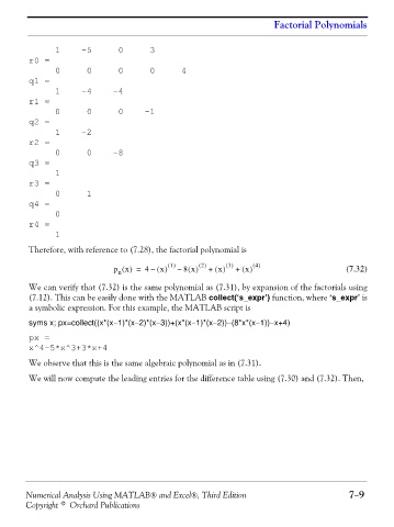
1 -5 0 3
r0 =
0 0 0 0 4
q1 =
1 -4 -4
r1 =
0 0 0 -1
q2 =
1 -2
r2 =
0 0 -8
q3 =
1
r3 =
0 1
q4 =
0
r4 =
1
Therefore, with reference to (7.28), the factorial polynomial is

p x() = 4 – x () 1 () – 8x() 2 () + x () 3 () + x () 4 () (7.32)
n
We can verify that (7.32) is the same polynomial as (7.31), by expansion of the factorials using
(7.12). This can be easily done with the MATLAB collect(‘s_expr’) function, where ‘s_expr’ is
a symbolic expression. For this example, the MATLAB script is

syms x; px=collect((x*(x−1)*(x−2)*(x−3))+(x*(x−1)*(x−2))−(8*x*(x−1))−x+4)

px =
x^4-5*x^3+3*x+4
We observe that this is the same algebraic polynomial as in (7.31).
We will now compute the leading entries for the difference table using (7.30) and (7.32). Then,

Numerical Analysis Using MATLAB® and Excel®, Third Edition 7−9
Copyright © Orchard Publications