Page 288 - Numerical Analysis Using MATLAB and Excel

Chapter 7 Finite Differences and Interpolation

0
⋅
Δ p0() = 0! 4 = 4
1
)
Δ p0() = 1! ( ⋅ – 1 = – 1
2
)
Δ p0() = 2! ( ⋅ – 8 = – 16
(7.33)
3
⋅
Δ p0() = 3! 1 = 6
4
⋅
Δ p0() = 4! 1 = 24
5
⋅
Δ p0() = 5! 0 = 0
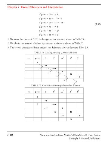
1. We enter the values of (7.33) in the appropriate spaces as shown in Table 7.6.
2. We obtain the next set of values by crisscross addition as shown in Table 7.7.
3. The second crisscross addition extends the difference table as shown in Table 7.8.

TABLE 7.6 Leading entries of (7.33) in table form

x p x() Δ Δ 2 Δ 3 Δ 4 Δ 5

4
−1
−16
6
24
0

TABLE 7.7 Crisscross addition to find second set of values

x p x() Δ Δ 2 Δ 3 Δ 4 Δ 5

4

−1
3 −16

−17 6
−10 24
30 0
24

7−10 Numerical Analysis Using MATLAB® and Excel®, Third Edition
Copyright © Orchard Publications