Page 280 - Numerical Analysis Using MATLAB and Excel

Chapter 7 Finite Differences and Interpolation

The third, fourth, and so on divided differences, are defined similarly.
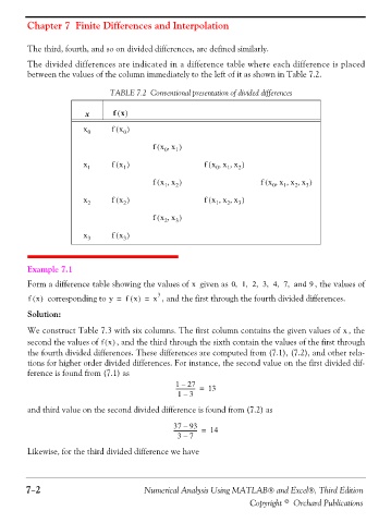
The divided differences are indicated in a difference table where each difference is placed
between the values of the column immediately to the left of it as shown in Table 7.2.

TABLE 7.2 Conventional presentation of divided differences

x fx()

x 0 fx ) ( 0

fx x,( 0 1 )

x 1 fx ) ( 1 fx x x ) ( 0 , 1 , 2

fx x,( 1 2 ) fx x x x ) ( 0 , 1 , 2 , 3

x 2 fx ) ( 2 fx x x ) ( 1 , 2 , 3

fx x,( 2 3 )

x 3 fx ) ( 3

Example 7.1
Form a difference table showing the values of given as 0 1 2 3 4 7 and 9, , , , , , , the values of
x
fx() corresponding to y = f x() = x 3 , and the first through the fourth divided differences.

Solution:
We construct Table 7.3 with six columns. The first column contains the given values of , the
x
second the values of fx() , and the third through the sixth contain the values of the first through
the fourth divided differences. These differences are computed from (7.1), (7.2), and other rela-
tions for higher order divided differences. For instance, the second value on the first divided dif-
ference is found from (7.1) as
1 – 27 13
--------------- =
1 – 3
and third value on the second divided difference is found from (7.2) as

–
37 93
------------------ = 14
–
37
Likewise, for the third divided difference we have

7−2 Numerical Analysis Using MATLAB® and Excel®, Third Edition
Copyright © Orchard Publications