Page 320 - Numerical Analysis Using MATLAB and Excel

Chapter 7 Finite Differences and Interpolation

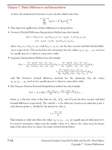
we have the fundamental theorem of sum calculus which states that

)
α + ( n – 1 h – α +
∑ p x() = Δ p x() nh
1
n
n
x = α α
• One important application of finite differences is interpolation.
• Newton’s Divided Difference Interpolation Method uses the formula

fx() = fx ) ( 0 + ( xx ) – 0 fx x ) ( 0 , 1 + ( x – x ) 0 ( xx ) – 1 fx x x ) ( 0 , 1 , 2
xx )+ ( – 0 ( x – x ) 1 ( x – x ) 2 fx x x x ) ( 0 , 1 , 2 , 3

where fx x,( 0 1 ) , fx x x,( 0 1 , 2 ) , and fx x x x,( 0 1 , 2 , 3 ) are the first, second, and third divided differ-

ences respectively. This method has the advantage that the values x x x … x, 0 1 , 2 , , n need not
be equally spaced, or taken in consecutive order.
• Lagrange’s Interpolation Method uses the formula

( x – x ) ( xx ) – … ( x – x ) ( xx ) – ( x – x ) … ( xx ) –
1
2
2
n
n
0
fx() = ------------------------------------------------------------------------fx ( ) + ------------------------------------------------------------------------fx ( )
( x – x ) 1 ( x – x ) 2 … ( x – x ) n 0 ( x – x ) 0 ( x – x ) 2 … ( x – x ) n 1
0
1
1
1
0
0
( x – x ) ( xx ) – … ( x – x )
n –
1
1
0
+ ------------------------------------------------------------------------------fx ( )
( x – x ) 0 ( x – x ) 2 … ( x – x n – 1 ) n
n
n
n
and, like Newton’s divided difference method, has the advantage that the values
x x x … x, 0 1 , 2 , , n need not be equally spaced or taken in consecutive order.
•The Gregory−Newton Forward Interpolation method uses the formula
(
(
(
)
rr – 1 ) 2 rr – 1 r – 2 ) 3
fx() = f + rΔf + ------------------Δ f + ----------------------------------Δ f + …
0
0
0
0
2!
3!
2 3
f
where is the first value of the data set, Δf 0 , Δ f 0 , and Δ f 0 are the first, second, and third
0
r
forward differences respectively. The variable is the difference between an unknown point x
and a known point x 1 divided by the interval , that is,
h
( x – x )
1
r = -------------------
h
This formula is valid only when the values x x x … x, 0 1 , 2 , , n are equally spaced with interval . h
It is used to interpolate values near the smaller values of , that is, the values near the begin-
x
ning of the given data set, hence the name forward interpolation.
7−42 Numerical Analysis Using MATLAB® and Excel®, Third Edition
Copyright © Orchard Publications