Page 23 - Numerical Methods for Chemical Engineering

12 1 Linear algebra

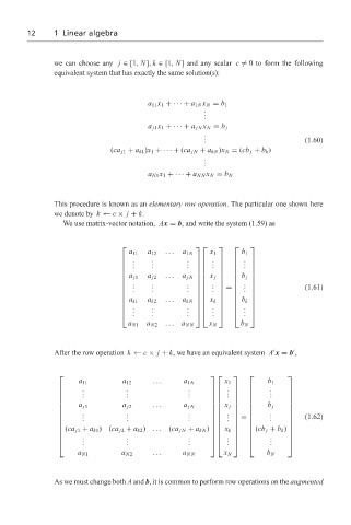
we can choose any j ∈ [1, N], k ∈ [1, N] and any scalar c = 0 to form the following
equivalent system that has exactly the same solution(s):

a 11 x 1 +· · · + a 1N x N = b 1
.
.
.
a j1 x 1 +· · · + a jN x N = b j
.
.
. (1.60)
(ca j1 + a k1 )x 1 +· · · + (ca jN + a kN )x N = (cb j + b k )
.
.
.
a N1 x 1 +· · · + a NN x N = b N

This procedure is known as an elementary row operation. The particular one shown here
we denote by k ← c × j + k.
We use matrix-vector notation, Ax = b, and write the system (1.59) as

     
a 11 a 12 ... a 1N x 1 b 1
 . .  . 
 . . .   . 
. . . .   .   . 
.
.
     
 ...     
 a j1 a j2 a jN   x j   b j 
 . . .   .   . 
 . . (1.61)
 . . .   .  =  . 
.   . 
 . 
     
 a k1 a k2 ... a kN   x k   b k 
 . .     

.
.
 . . . . . .   .   . 
.   . 
 . 
a N1 a N2 ... a NN x N b N
After the row operation k ← c × j + k, we have an equivalent system A x = b ,

  
  
a 11 a 12 ... a 1N x 1 b 1
. . . .
 . . .   .   . 
. . . . .
   .   
     
     
a j1 a j2 ... a jN b j
   x j   
 . . .   .   . 
. . . .
 . . .   .  =  .  (1.62)
   .   
 (ca j1 + a k1 )(ca j2 + a k2 ) ... (ca jN + a kN )   x k   

 

 (cb j + b k ) 
. . . .
     
.
 . . .   .   . 
 . . .   .   . 
...
a N1 a N2 a NN x N b N
As we must change both A and b, it is common to perform row operations on the augmented