Page 24 - Numerical Methods for Chemical Engineering

Elimination methods for solving linear systems 13

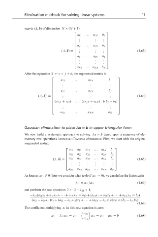
matrix (A, b) of dimension N × (N + 1),
 
...
a 11 a 1N b 1
 . .
 . . . 
. . . . 
 
 ... 
 a j1 a jN b j 
 . . . 
 .
(A, b) =  . . . .  (1.63)
. 
 
 a k1 ... a kN b k 
 . . 

 . . . . . . 
. 
a N1 ... a NN b N
After the operation k ← c × j + k, the augmented matrix is
 
...
a 11 a 1N b 1
. . .
 . . . 
. . .
 
 
 
a j1 ... a jN b j
 
 . . . 

(A, b) =  . . . . . .  (1.64)
 
 
 (ca j1 + a k1 )
... (ca jN + a kN )(cb j + b k ) 
. . .
 
 . . . 
 . . . 
a N1 ... a NN b N
Gaussian elimination to place Ax = b in upper triangular form
We now build a systematic approach to solving Ax = b based upon a sequence of ele-
mentary row operations, known as Gaussian elimination. First, we start with the original
augmented matrix
 
a 11 a 12 a 13 ... a 1N b 1
...
 a 21 a 22 a 23 a 2N b 2 
 
a 31 a 32 a 33 a 3N (1.65)
 ... 
(A, b) =  b 3 
 . . . . .
 . . . . . . . . . . . 
.
. 
a N1 a N2 a N3 ... a NN b N
As long as a 11 = 0 (later we consider what to do if a 11 = 0), we can define the finite scalar
λ 21 = a 21 /a 11 (1.66)
and perform the row operation 2 ← 2 − λ 21 × 1,
−λ 21 (a 11 x 1 + a 12 x 2 +· · · + a 1N x N = b 1 ) + (a 21 x 1 + a 22 x 2 +· · · + a 2N x N = b 2 )
(a 21 − λ 21 a 11 )x 1 + (a 22 − λ 21 a 12 )x 2 + ··· + (a 2N − λ 21 a 1N )x N = (b 2 − λ 21 b 1 )
(1.67)
The coefficient multiplying x 1 in this new equation is zero:

a 21
a 21 − λ 21 a 11 = a 21 − a 11 = a 21 − a 21 = 0 (1.68)
a 11