Page 247 - Numerical Methods for Chemical Engineering

236 5 Numerical optimization

2
1

−1
−2
−2 2

Figure 5.12 Trajectory of multiplier iterations when finding the closest points on two ellipses.

x x
1 easie set 2
∇ 2
inactive
active 1
1 2 inactive
inactive
2
∇ 1 1 inactive
2 active
ineasie
ineasie

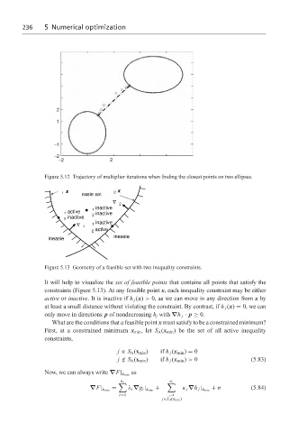
Figure 5.13 Geometry of a feasible set with two inequality constraints.
It will help to visualize the set of feasible points that contains all points that satisfy the
constraints (Figure 5.13). At any feasible point x, each inequality constraint may be either
active or inactive. It is inactive if h j (x) > 0, as we can move in any direction from x by
at least a small distance without violating the constraint. By contrast, if h j (x) = 0, we can
only move in directions p of nondecreasing h j with ∇h j · p ≥ 0.
What are the conditions that a feasible point x must satisfy to be a constrained minimum?
First, at a constrained minimum x min , let S A (x min ) be the set of all active inequality
constraints,
j ∈ S A (x min ) if h j (x min ) = 0
j /∈ S A (x min ) if h j (x min ) > 0 (5.83)

as
Now, we can always write ∇F| x min
= n e + n i + v (5.84)
∇F| x min λ i ∇g i | x min κ j ∇h j | x min
i=1 j=1
j∈S A (x min )