Page 244 - Numerical Methods for Chemical Engineering

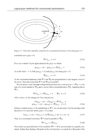
Lagrangian methods for constrained optimization 233

x

cnstrained V λV ∆
ini
∆
v V ∆ v

Figure 5.11 First-order optimality conditions for a constrained minimum of F(x) along g(x) = 0.

constraint curve g(x) = 0,
· t = 0 (5.62)
∇F| x min
If we use a similar Taylor approximation for g(x), we obtain
· t (5.63)
g(x min + εt) − g(x min ) = ε∇g| x min
As in the limit ε → 0, both g(x min + εt) and g(x min ) lie along g(x) = 0,
· t = 0 (5.64)
∇g| x min
At the constrained minimum, both ∇F and ∇g are perpendicular to any tangent vector of
the curve. Does that mean that ∇F and ∇g are parallel?
We can always write (through orthogonal projection) any vector p as p = λ∇g + v, the
sum of a vector parallel to ∇g and a vector v that is perpendicular to ∇g. Applying this to
∇F,

+ v ∇g · v = 0 (5.65)
∇F| x min = λ∇g| x min
After a move εv, the changes in F(x) and g(x) are

· v
F(x min + εv) − F(x min ) = ε∇F| x min
· v = 0 (5.66)
g(x min + εv) − g(x min ) = ε∇g| x min
If there is indeed some v = 0 contributing to ∇F, we can decrease F(x) by moving in the
direction of ±v and still satisfy g(x) = 0, as then
F(x min + εv) − F(x min ) = ε[λ∇g|x min + v] · v = ε(v · v) (5.67)

Thus, at a constrained minimum, ∇F must be parallel to ∇g,
(5.68)
∇F| x min = λ∇g| x min
This yields our generalization of the condition ∇F = 0 to accommodate an equality con-
straint. Rather than finding a flat point in the cost function, we search for a flat point of the