Page 241 - Numerical Methods for Chemical Engineering

230 5 Numerical optimization

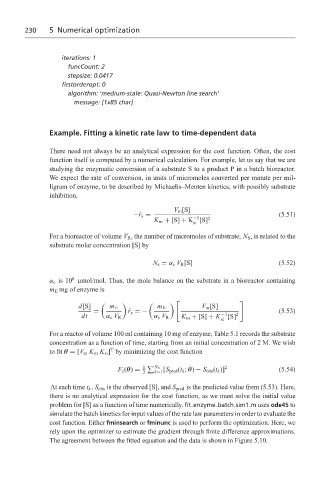
iterations: 1
funcCount: 2
stepsize: 0.0417
firstorderopt: 0
algorithm: ‘medium-scale: Quasi-Newton line search’
message: [1x85 char]

Example. Fitting a kinetic rate law to time-dependent data

There need not always be an analytical expression for the cost function. Often, the cost
function itself is computed by a numerical calculation. For example, let us say that we are
studying the enzymatic conversion of a substrate S to a product P in a batch bioreactor.
We expect the rate of conversion, in units of micromoles converted per minute per mil-
ligram of enzyme, to be described by Michaelis–Menten kinetics, with possibly substrate
inhibition,

V m [S]
−ˆ r s = −1 (5.51)
K m + [S] + K [S] 2
si
For a bioreactor of volume V R , the number of micromoles of substrate, N S , is related to the
substrate molar concentration [S] by

N s = α c V R [S] (5.52)

6
α c is 10 µmol/mol. Thus, the mole balance on the substrate in a bioreactor containing
m E mg of enzyme is

d[S] m E m E V m [S]

= ˆ r s =− (5.53)
dt α c V R α c V R K m + [S] + K −1 [S] 2
si
For a reactor of volume 100 ml containing 10 mg of enzyme, Table 5.1 records the substrate
concentration as a function of time, starting from an initial concentration of 2 M. We wish
T
to fit θ = [V m K m K si ] by minimizing the cost function
1 N d 2
F c (θ) = [S pred (t k ; θ) − S obs (t k )] (5.54)
2 k=1
At each time t k , S obs is the observed [S], and S pred is the predicted value from (5.53). Here,
there is no analytical expression for the cost function, as we must solve the initial value
problem for [S] as a function of time numerically. fit enzyme batch sim1.m uses ode45 to
simulate the batch kinetics for input values of the rate law parameters in order to evaluate the
cost function. Either fminsearch or fminunc is used to perform the optimization. Here, we
rely upon the optimizer to estimate the gradient through finite difference approximations.
The agreement between the fitted equation and the data is shown in Figure 5.10.