Page 237 - Numerical Methods for Chemical Engineering

226 5 Numerical optimization

p c p d a r i n
0 r d e
et d p s
s = 1 c
∆ s =

p s
p n
s 2

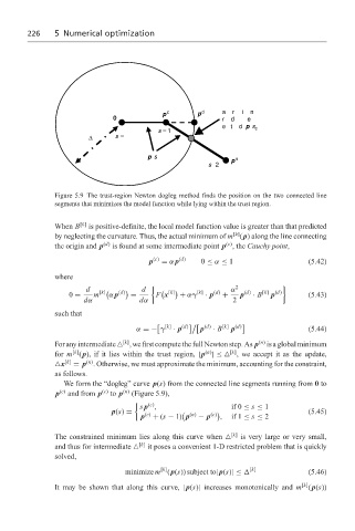
Figure 5.9 The trust-region Newton dogleg method finds the position on the two connected line
segments that minimizes the model function while lying within the trust region.

When B [k] is positive-definite, the local model function value is greater than that predicted
[k]
by neglecting the curvature. Thus, the actual minimum of m (p) along the line connecting
(c)
the origin and p (d) is found at some intermediate point p , the Cauchy point,
p (c) = α p (d) 0 ≤ α ≤ 1 (5.42)

where
d [k] (d) d [k] [k] (d) α 2 (d) [k] (d) 1
0 = m α p = F x + αγ · p + p · B p (5.43)
dα dα 2
such that

α =− γ [k] · p (d) p (d) · B [k] p (d) (5.44)
[k]
For any intermediate , we first compute the full Newton step. As p (n) is a global minimum
[k]
[k]
(n)
for m (p), if it lies within the trust region, |p |≤ , we accept it as the update,
(n)
x [k] = p . Otherwise, we must approximate the minimum, accounting for the constraint,
as follows.
We form the “dogleg” curve p(s) from the connected line segments running from 0 to
p (c) and from p (c) to p (n) (Figure 5.9),
s p , if 0 ≤ s ≤ 1
(c)
p(s) = (c) (n) (c) (5.45)
p + (s − 1) p − p , if 1 ≤ s ≤ 2
[k]
The constrained minimum lies along this curve when is very large or very small,
[k]
and thus for intermediate it poses a convenient 1-D restricted problem that is quickly
solved,
[k]
minimize m (p(s)) subject to|p(s)|≤ [k] (5.46)
[k]
It may be shown that along this curve, |p(s)| increases monotonically and m (p(s))