Page 232 - Numerical Methods for Chemical Engineering

Gradient methods 221

γ 1
x 1

p
x

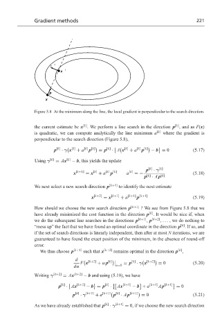
Figure 5.8 At the minimum along the line, the local gradient is perpendicular to the search direction.

[k]
[k]
the current estimate be x . We perform a line search in the direction p , and as F(x)
is quadratic, we can compute analytically the line minimum a [k] where the gradient is
perpendicular to the search direction (Figure 5.8),

p
p
p [k] · γ x [k] + a [k] [k] = p [k] · A x [k] + a [k] [k] − b = 0 (5.17)
Using γ [k] = Ax [k] − b, this yields the update
p [k] · γ [k]
[k+1] [k] [k] [k] [k]
x = x + a p a =− (5.18)
p [k] · Ap [k]
We next select a new search direction p [k+1] to identify the next estimate
x [k+2] = x [k+1] + a [k+1] [k+1] (5.19)
p
How should we choose the new search direction p [k+1] ? We see from Figure 5.8 that we
[k]
have already minimized the cost function in the direction p . It would be nice if, when
we do the subsequent line searches in the directions p [k+1] , p [k+2] ,... , we do nothing to
[k]
“mess up” the fact that we have found an optimal coordinate in the direction p . If so, and
if the set of search directions is linearly independent, then after at most N iterations, we are
guaranteed to have found the exact position of the minimum, in the absence of round-off
error.
[k]
We thus choose p [k+1] such that x [k+2] remains optimal in the direction p ,
d [k+2] [k] [k+2]
F x + α p [k] = p · γ x = 0 (5.20)
dα α=0
Writing γ [k+2] = Ax [k+2] − b and using (5.19), we have

p [k] · Ax [k+2] − b = p [k] · Ax [k+1] − b + a [k+1] Ap [k+1] = 0
p [k] · γ [k+1] + a [k+1] p [k] · Ap [k+1] = 0 (5.21)
As we have already established that p [k] · γ [k+1] = 0, if we choose the new search direction