Page 228 - Numerical Methods for Chemical Engineering

Gradient methods 217

x in

x 1 x

d
x 2
x

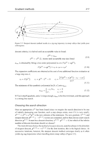
Figure 5.5 Steepest descent method results in a zig-zag trajectory in steep valleys that yields poor
convergence.

descent criteria, it is halved until an acceptable value is found:

a [k] = a max
(5.9)
[k]
a [k] ← a /2, iterate until acceptable step size found
[k]
a max is obtained by fitting a low-order polynomial in a to F(x [k] + a p ),
[k] [k] 2
F x + a p ≈ c 0 + c 1 a + c 2 a (5.10)
The expansion coefficients are obtained at the cost of one additional function evaluation at
a large step size a ,
[k] [k]
F x + a p − c 0 − c 1 a
[k] [k] [k]
c 0 = F x c 1 = p · γ < 0 c 2 =
2
(a )
(5.11)

The minimum of this quadratic polynomial in [0, a ] sets a max ,

−c 1 /2c 2 , c 2 > 0
a max = (5.12)

a , c 2 ≤ 0
If F(x) is itself quadratic, and a is large enough, a max is the line minimum, and this approach

is a strong line search.
Choosing the search direction
Once an appropriate a [k] has been found (since we require the search direction to be one
of initially decreasing cost function, such a step always exists, even if it is very small),
x [k+1] = x [k] + a [k] [k] is the new estimate of the minimum. The new gradient, γ [k+1] , and
p
steepest descent, d [k+1] =−γ [k+1] , vectors are computed, and we then choose a new search
direction p [k+1] . It must be a descent direction, γ [k+1] · p [k+1] < 0, but which of the infinite
number of descent directions should we choose?
The most obvious choice, the method of steepest descent, searches always in the direction
of steepest descent, p [k+1] =−γ [k+1] . For the first iteration, this is the logical choice. At
successive iterations, however, the steepest descent method converges slowly as it often
yields zig-zag trajectories when travelling down steep valleys (Figure 5.5).