Page 224 - Numerical Methods for Chemical Engineering

Gradient methods 213

we move to it from x [0] by descending “downhill” until we cannot decrease F(x)any
further.
To use these methods, we must supply at least a routine that returns the cost function
value F(x) for an input x. Gradient methods in addition require knowledge of the gradient
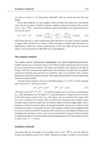
vector γ(x) = ∇F| x , and Newton methods require knowledge (or an approximation) of
the Hessian matrix
2 2
2
H =∇ F = H T H jk (x) = ∂ F = ∂γ k = ∂ F = H kj (x) (5.2)

∂x j ∂x k x ∂x j x ∂x k ∂x j x
While these derivatives can be estimated by finite differences, for large systems it is helpful
to supply them directly for an input x. With knowledge of higher-order derivatives, an
optimization routine has a better understanding of the local shape of the cost function
surface, and can search more efficiently for a local minimum.

The simplex method

The simplex method, implemented as fminsearch in the optional MATLAB optimization
toolkit,requiresonlyaroutinethatreturns F(x).Whilesimplexmethodsareusedcommonly
for linear programming problems with linear cost functions and constraints (Nocedal &
Wright, 1999), for unconstrained optimization with nonlinear cost functions, the gradient
and Newton methods discussed below are preferred. Thus, we provide here only a cursory
description, and refer the interested reader to the supplemental material in the accompanying
website for further details.
2
The basic idea is easiest to see for a 2-D problem (Figure 5.1). In , we form a triangle
with vertices at x [0] and the two points

x [1] = x [0] + l 1 e [1] x [2] = x [0] + l 2 e [2] (5.3)
[2]
[0]
[1]
We want to move {x , x , x ,...} so that the triangle comes to enclose a local minimum
x min while shrinking in size. In Figure 5.1, a typical sequence of simplex moves is shown,
if the farther away a point is from x min , the higher is its cost function. First (upper left),
the vertex of highest cost function value is moved in the direction of the triangle’s center
towards a region where we expect the cost function values to be lower (upper right). After a
sequence of such moves (lower right), the triangle eventually contains in its interior a local
minimum (we hope). At this point, the size of the triangle is reduced until it tightly bounds
the local minimum (lower left). In practice, both vertex moves and triangle shrinking occur
throughout the calculation, as the vertex moves are most likely to succeed when the triangle
N
is small enough that F(x) varies linearly over the triangle region. In the triangle becomes
a simplex with N + 1 vertices.

Gradient methods

Algorithms that use knowledge of the gradient vector γ(x) = ∇F| x are more efficient,
because the gradient points in the “uphill” direction of steepest increase in cost function