Page 225 - Numerical Methods for Chemical Engineering

214 5 Numerical optimization

x in x in

x 2 x 1 x 2

x x 1 x

x 2
x in
x 2 x in
x
x
x 1
x 1

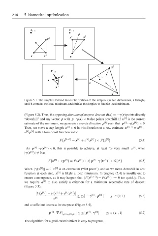
Figure 5.1 The simplex method moves the vertices of the simplex (in two dimensions, a triangle)
until it contains the local minimum, and shrinks the simplex to find the local minimum.

(Figure 5.2). Thus, the opposing direction of steepest descent d(x) =−γ(x) points directly
“downhill” and any vector p with p · γ(x) < 0 also points downhill. If x [k] is the current
[k]
estimate of the minimum, we generate a search direction p [k] such that p [k] · γ(x ) < 0.
Then, we move a step length a [k] > 0 in this direction to a new estimate x [k+1] = x [k] +
a [k] [k] with a lower cost function value
p
[k+1] [k] [k] [k] [k]
F x = x + a p < F x (5.4)
[k]
[k]
As p [k] · γ(x ) < 0, this is possible to achieve, at least for very small a , when
[k]
|γ(x )| = 0as
[k] [k] [k] [k] [k] 2
F x + εp = F x + ε p · γ x + O[ε ] (5.5)
[k]
When |γ(x )|= 0, x [k] is an extremum (“flat point”), and as we move downhill in cost
function at each step, x [k] is likely a local minimum. In practice (5.4) is insufficient to
[k]
ensure convergence, as it may happen that |F(x [k+1] ) − F(x )|→ 0 too quickly. Thus,
we require a [k] to also satisfy a criterion for a minimum acceptable rate of descent
(Figure 5.3),

[k] [k]
F x − F x + a p
[k] [k] [k] [k]
≥ χ 1 − γ · p χ 1 ∈ (0, 1) (5.6)
a [k]
and a sufficient decrease in steepness (Figure 5.4),
[k]
[k] · ∇F [k] ≤ χ 2 p · γ [k] χ 2 ∈ (χ 1 , 1) (5.7)

p
[k]

x +a [k] p
The algorithm for a gradient minimizer is easy to program,