Page 231 - Numerical Methods for Chemical Engineering

220 5 Numerical optimization

1 1

initia ess iter = initia ess iter = 1
2 2

− −
− 1 − 1
1 1
1 1

initia ess iter = initia ess iter = 2
2 2

− −
− 1 − 1
1 1
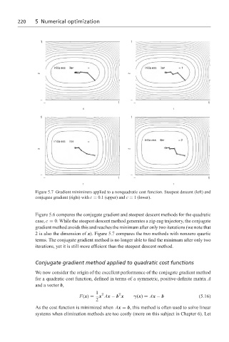
Figure 5.7 Gradient minimizers applied to a nonquadratic cost function. Steepest descent (left) and
conjugate gradient (right) with c = 0.1 (upper) and c = 1 (lower).

Figure 5.6 compares the conjugate gradient and steepest descent methods for the quadratic
case, c = 0. While the steepest descent method generates a zig-zag trajectory, the conjugate
gradient method avoids this and reaches the minimum after only two iterations (we note that
2 is also the dimension of x). Figure 5.7 compares the two methods with nonzero quartic
terms. The conjugate gradient method is no longer able to find the minimum after only two
iterations, yet it is still more efficient than the steepest descent method.

Conjugate gradient method applied to quadratic cost functions

We now consider the origin of the excellent performance of the conjugate gradient method
for a quadratic cost function, defined in terms of a symmetric, positive-definite matrix A
and a vector b,
1 T T
F(x) = x Ax − b x γ(x) = Ax − b (5.16)
2
As the cost function is minimized when Ax = b, this method is often used to solve linear
systems when elimination methods are too costly (more on this subject in Chapter 6). Let