Page 55 - Numerical Methods for Chemical Engineering

44 1 Linear algebra

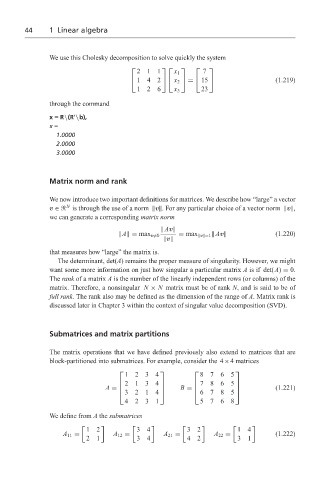
We use this Cholesky decomposition to solve quickly the system
211 x 1 7
     
142 = 15 (1.219)
   x 2   
126 x 3 23
through the command

x = R\(R \b),
x =
1.0000
2.0000
3.0000

Matrix norm and rank

We now introduce two important definitions for matrices. We describe how “large” a vector
N
v ∈ is through the use of a norm v . For any particular choice of a vector norm v ,
we can generate a corresponding matrix norm

Av
A = max v =0 = max v =1 Av (1.220)
v
that measures how “large” the matrix is.
The determinant, det(A) remains the proper measure of singularity. However, we might
want some more information on just how singular a particular matrix A is if det(A) = 0.
The rank of a matrix A is the number of the linearly independent rows (or columns) of the
matrix. Therefore, a nonsingular N × N matrix must be of rank N, and is said to be of
full rank. The rank also may be defined as the dimension of the range of A. Matrix rank is
discussed later in Chapter 3 within the context of singular value decomposition (SVD).

Submatrices and matrix partitions

The matrix operations that we have defined previously also extend to matrices that are
block-partitioned into submatrices. For example, consider the 4×4 matrices

1234 8765
   
2134 7865
   
A =   B =   (1.221)
 3214   6785 
4231 5768
We define from A the submatrices

12 34 32 14
A 11 = A 12 = A 21 = A 22 = (1.222)
21 34 42 31