Page 56 - Numerical Methods for Chemical Engineering

Example. Modeling a separation system 45

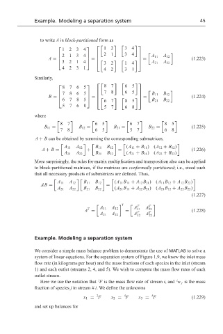
to write A in block-partitioned form as
 
1234
  12 34
2134  21 34 
  A 11 A 12
 
A =    = (1.223)
3214 = 
  A 21 A 22
 32 14 
4231 42 31
Similarly,
 
  87 65
8765
7865  78 65 
  B 11 B 12
 
B =    = (1.224)
6785 = 
  B 21 B 22
 67 85 
5768 57 68
where

87 65 67 85
B 11 = B 12 = B 21 = B 22 = (1.225)
78 65 57 68
A + B can be obtained by summing the corresponding submatrices,

A 11 A 12 B 11 B 12 (A 11 + B 11 )(A 12 + B 12 )
A + B = + = (1.226)
A 21 A 22 B 21 B 22 (A 21 + B 21 )(A 22 + B 22 )
More surprisingly, the rules for matrix multiplication and transposition also can be applied
to block-partitioned matrices, if the matrices are conformally partitioned; i.e., sized such
that all necessary products of submatrices are defined. Thus,

A 11 A 12 B 11 B 12 (A 11 B 11 + A 12 B 21 )(A 11 B 12 + A 12 B 22 )
AB = =
A 21 A 22 B 21 B 22 (A 21 B 11 + A 22 B 21 )(A 21 B 12 + A 22 B 22 )
(1.227)
T
T T
A A
T A 11 A 12 11 21
A = = T T (1.228)
A 21 A 22 A A
12 22

Example. Modeling a separation system

We consider a simple mass balance problem to demonstrate the use of MATLAB to solve a
system of linear equations. For the separation system of Figure 1.9, we know the inlet mass
flow rate (in kilograms per hour) and the mass fractions of each species in the inlet (stream
1) and each outlet (streams 2, 4, and 5). We wish to compute the mass flow rates of each
outlet stream.
i
i
Here we use the notation that F is the mass flow rate of stream i, and w j is the mass
fraction of species j in stream #i. We define the unknowns
5
2
4
x 1 = F x 2 = F x 3 = F (1.229)
and set up balances for