Page 59 - Numerical Methods for Chemical Engineering

48 1 Linear algebra

. . . . B

. . . . . 1 ∆

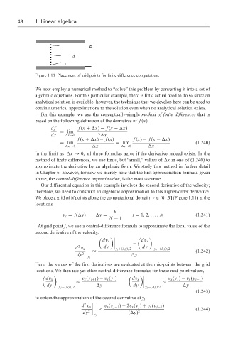
Figure 1.11 Placement of grid points for finite difference computation.

We now employ a numerical method to “solve” this problem by converting it into a set of
algebraic equations. For this particular example, there is little actual need to do so since an
analytical solution is available; however, the technique that we develop here can be used to
obtain numerical approximations to the solution even when no analytical solution exists.
For this example, we use the conceptually-simple method of finite differences that is
based on the following definition of the derivative of f (x):
df f (x + x) − f (x − x)
= lim
dx x→0 2 x
f (x + x) − f (x) f (x) − f (x − x)
= lim = lim (1.240)
x→0 x x→0 x
In the limit as x → 0, all three formulas agree if the derivative indeed exists. In the
method of finite differences, we use finite, but “small,” values of x in one of (1.240) to
approximate the derivative by an algebraic form. We study this method in further detail
in Chapter 6; however, for now we merely note that the first approximation formula given
above, the central-difference approximation, is the most accurate.
Our differential equation in this example involves the second derivative of the velocity;
therefore, we need to construct an algebraic approximation to this higher-order derivative.
We place a grid of N points along the computational domain y ∈ [0, B] (Figure 1.11) at the
locations
B
y j = j( y) y = j = 1, 2,..., N (1.241)
N + 1
At grid point j, we use a central-difference formula to approximate the local value of the
second derivative of the velocity,

dv x dv x
−
2 dy dy
d v x y j +( y)/2 y j −( y)/2
≈ (1.242)
dy 2 y
y j
Here, the values of the first derivatives are evaluated at the mid-points between the grid
locations. We then use yet other central-difference formulas for these mid-point values,

dv x v x (y j+1 ) − v x (y j ) dv x v x (y j ) − v x (y j−1 )
≈ ≈
dy y dy y
y j +( y)/2 y j −( y)/2
(1.243)
to obtain the approximation of the second derivative at y j
2
d v x v x (y j+1 ) − 2v x (y j ) + v x (y j−1 )
≈ (1.244)
dy 2 ( y) 2
y j