Page 62 - Numerical Methods for Chemical Engineering

Sparse and banded matrices 51

2 −1
 
 −1 2 −1 
A =   (1.254)
−1 2 −1
 
−1 2
can be stored as

1 1 2 a 11 = 2
     
1 2 −1 a 12 =−1
     
     
2
1
     −1  a 21 =−1
     
a 22 = 2
     
 2   2   2 
a 23 =−1
     
 2   3   −1 
⇔ (1.255)
a 32 =−1
i row =  
j col =  
a = 

 3   2   −1 
     
a 33 = 2
 3   3   2 
     
3 4 −1 a 34 =−1
     
     
3
4
     −1  a 43 =−1
4 4 2 a 44 = 2
Obviously, this format requires much less memory for sparse matrices than does allocating
a separate location to store a real value for each element, whether it is zero or not.
Even though it is possible to store a sparse matrix efficiently, can we efficiently solve a
system by Gaussian elimination using this notation? We can if the matrix is banded; i.e., if
the nonzero values are clustered in the vicinity of the principal diagonal.
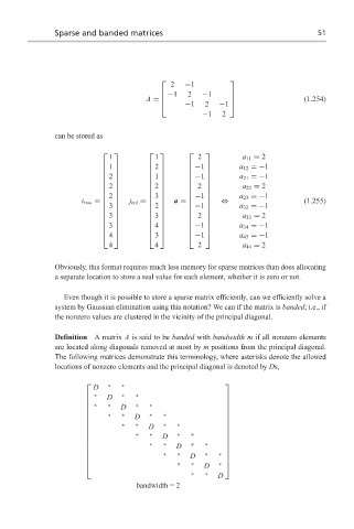
Definition A matrix A is said to be banded with bandwidth m if all nonzero elements
are located along diagonals removed at most by m positions from the principal diagonal.
The following matrices demonstrate this terminology, where asterisks denote the allowed
locations of nonzero elements and the principal diagonal is denoted by Ds,
D
 ∗ ∗ 
 ∗ D ∗ ∗ 
 
 ∗ ∗ D ∗ ∗ 


D
 ∗ ∗ ∗ ∗ 
 
∗ ∗ D ∗ ∗
 
 
∗ ∗ D ∗ ∗
 
 
 
∗ ∗ D ∗ ∗
 
 
∗ ∗ ∗
 D ∗ 
 
∗ ∗
 D ∗ 
∗ ∗ D
bandwidth = 2