Page 64 - Numerical Methods for Chemical Engineering

Sparse and banded matrices 53

1

1

2

2
1 1 2 2
n
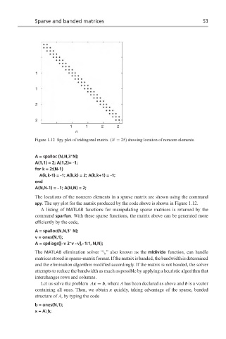
Figure 1.12 Spy plot of tridiagonal matrix (N = 25) showing location of nonzero elements.

∗
A = spalloc (N,N,3 N);
A(1,1) = 2; A(1,2)= -1;
for k = 2:(N-1)
A(k,k-1) = -1; A(k,k) = 2; A(k,k+1) = -1;
end
A(N,N-1) = - 1; A(N,N) = 2;
The locations of the nonzero elements in a sparse matrix are shown using the command
spy. The spy plot for the matrix produced by the code above is shown in Figure 1.12.
A listing of MATLAB functions for manipulating sparse matrices is returned by the
command sparfun. With these sparse functions, the matrix above can be generated more
efficiently by the code,
A = spalloc(N,N,3 N);
∗
v = ones(N,1);
A = spdiags([- v 2 v - v],- 1:1, N,N);
∗
The MATLAB elimination solver “\,” also known as the mldivide function, can handle
matrices stored in sparse-matrix format. If the matrix is banded, the bandwidth is determined
and the elimination algorithm modified accordingly. If the matrix is not banded, the solver
attempts to reduce the bandwidth as much as possible by applying a heuristic algorithm that
interchanges rows and columns.
Let us solve the problem Ax = b, where A has been declared as above and b is a vector
containing all ones. Then, we obtain x quickly, taking advantage of the sparse, banded
structure of A, by typing the code
b = ones(N,1);
x=A\b;