Page 63 - Numerical Methods for Chemical Engineering

52 1 Linear algebra

D
 ∗ ∗ ∗ 
 ∗ D ∗ ∗ ∗ 
 
 ∗ ∗ D ∗ ∗ ∗ 
 
D
 ∗ ∗ ∗ ∗ ∗ ∗ 
 
D
 ∗ ∗ ∗ ∗ ∗ ∗ 
 
∗ ∗ ∗ D ∗ ∗ ∗
 
 
∗ ∗ ∗ ∗ ∗ ∗
 
 D 
 
∗ ∗ ∗ ∗ ∗
 D 
 
∗ ∗ ∗ ∗
 D 
D
∗ ∗ ∗
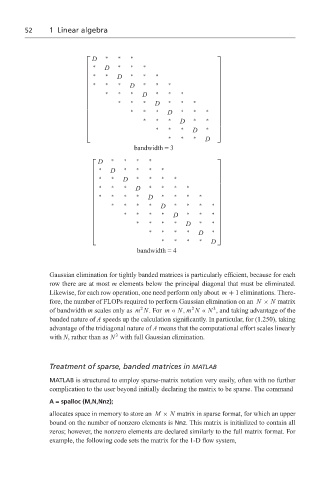
bandwidth = 3
D ∗ ∗ ∗ ∗
 
 ∗ D ∗ ∗ ∗ ∗ 
 
D 
 ∗ ∗ ∗ ∗ ∗ ∗
 
 ∗ ∗ ∗ D ∗ ∗ ∗ ∗ 
 
 ∗ ∗ ∗ ∗ D ∗ ∗ ∗ ∗ 
 
∗ ∗ ∗ ∗ D ∗ ∗ ∗ ∗
 
 
 
∗ ∗ ∗ ∗ ∗ ∗ ∗
 D 
 
∗ ∗ ∗ ∗ ∗
 D ∗ 
 
∗ ∗ ∗ ∗
 D ∗ 
D
∗ ∗ ∗ ∗
bandwidth = 4
Gaussian elimination for tightly banded matrices is particularly efficient, because for each
row there are at most m elements below the principal diagonal that must be eliminated.
Likewise, for each row operation, one need perform only about m + 1 eliminations. There-
fore, the number of FLOPs required to perform Gaussian elimination on an N × N matrix
3
2
2
of bandwidth m scales only as m N.For m « N, m N « N , and taking advantage of the
banded nature of A speeds up the calculation significantly. In particular, for (1.250), taking
advantage of the tridiagonal nature of A means that the computational effort scales linearly
3
with N, rather than as N with full Gaussian elimination.
Treatment of sparse, banded matrices in MATLAB
MATLAB is structured to employ sparse-matrix notation very easily, often with no further
complication to the user beyond initially declaring the matrix to be sparse. The command
A = spalloc (M,N,Nnz);
allocates space in memory to store an M × N matrix in sparse format, for which an upper
bound on the number of nonzero elements is Nnz. This matrix is initialized to contain all
zeros; however, the nonzero elements are declared similarly to the full matrix format. For
example, the following code sets the matrix for the 1-D flow system,