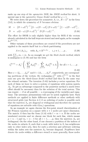
Page 228 -

5.1. Linear Stationary Iterative Methods 211

make up one step of the symmetric SOR,the SSOR method for short. A
special case is the symmetric Gauss–Seidel method for ω =1.
T
We write down the procedure for symmetric A, i.e., R = L in the form
(5.6), in which the symmetry of N becomes obvious:
T −1 & ' −1 & T '
M = D + ωL (1 − ω)D − ωL (D + ωL) (1 − ω)D − ωL ,
T −1 −1
N = ω(2 − ω) D + ωL D (D + ωL) . (5.38)
The effort for SSOR is only slightly higher than for SOR if the vectors
already calculated in the half steps are stored and used again, as for example
Lx (k+1/2) .
Other variants of these procedures are created if the procedures are not
applied to the matrix itself but to a block partitioning

with A ij ∈ R m i ,m j , i, j =1,...,p , (5.39)
A =(A ij ) i,j
p
with m i = m.As an example we get the block-Jacobi method,which
i=1
is analogous to (5.19) and has the form
 
i−1 p

(k+1) −1 (k) (k)
ξ i = A ii  − A ij ξ j − A ij ξ j + β i  for all i =1,... ,p.
j=1 j=i+1
(5.40)
T
T
Here x =(ξ 1 ,... ,ξ p ) and b =(β 1 ,...,β p ) , respectively, are correspond-
(k) (k+1)
ing partitions of the vectors. By exchanging ξ with ξ in the first
j j
sum one gets the block-Gauss–Seidel method and theninthe same way
the relaxed variants. The iteration (5.40) includes p vector equations. For
each of them we have to solve a system of equations with system matrix
A ii . To get an advantage compared to the pointwise method a much lower
effort should be necessary than for the solution of the total system. This
can require — if at all possible — a rearranging of the variables and equa-
tions. The necessary permutations will not be noted explicitly here. Such
methods are applied in finite difference methods or other methods with
structured grids (see Section 4.1) if an ordering of nodes is possible such
that the matrices A ii are diagonal or tridiagonal and therefore the systems
of equations are solvable with O(m i )operations.
As an example we again discuss the five-point stencil discretization of
the Poisson equation on a square with n + 1 nodes per space dimension.
The matrix A then has the form (1.14) with l = m = n. If the nodes are
numbered rowwise and we choose one block for each line, which means
p = n − 1and m i = n − 1 for all i =1,... ,p, then the matrices A ii are
tridiagonal. On the other hand, if one chooses a partition of the indices of
the nodes in subsets S i such that a node with index in S i has neighbours
only in other index sets, then for such a selection and arbitrary ordering
within the index sets the matrices A ii become diagonal. Neighbours here
denote the nodes within a difference stencil or more generally, those nodes