Page 231 -

214 5. Iterative Methods for Systems of Linear Equations


2 2 1/2
 1 ω β
 2 2
 1 − ω + ω β + ωβ 1 − ω +

 2 4
(2) (M SOR(ω) )=
for 0 <ω < ω opt





ω − 1 for ω opt ≤ ω< 2 ,
β 2
(3) M SOR(ω opt ) = 2 1/2 2 .
(1 + (1 − β ) )
Proof: See [18, p. 216].

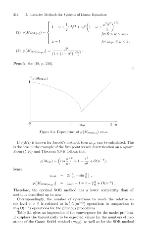
ρ( M SOR(ω) )
1

0 1 ω opt 2 ω

Figure 5.3. Dependence of M SOR(ω) on ω.

If (M J ) is known for Jacobi’s method, then ω opt can be calculated. This
is the case in the example of the five-point stencil discretization on a square:
From (5.26) and Theorem 5.9 it follows that
π π −4
2 2
(M GS )= cos =1 − + O(n );
n n 2
hence
π
ω opt = 2/ 1+sin n ,
π −2
= ω opt − 1= 1 − 2 + O(n ) .
M SOR(ω opt )
n
Therefore, the optimal SOR method has a lower complexity than all
methods described up to now.
Correspondingly, the number of operations to reach the relative er-
1
ror level ε> 0 is reduced to ln O(m 3/2 ) operations in comparison to
ε
1
2
ln O(m ) operations for the previous procedures.
ε
Table 5.1 gives an impression of the convergence for the model problem.
It displays the theoretically to be expected values for the numbers of iter-
ations of the Gauss–Seidel method (m GS ), as well as for the SOR method