Page 229 -

212 5. Iterative Methods for Systems of Linear Equations

 
4 −1 0 −1 0 0 0 0 0
 −1 4 −1 0 −1 0 0 0 0 
 
 0 −1 4 0 0 −1 0 0 0 
 
 −1 0 0 4 −1 0 −1 0 0 
 
 0 −1 0 −1 4 −1 0 −1 0 
 
 0 0 −1 0 −1 4 0 0 −1 
 
 0 0 0 −1 0 0 4 −1 0 
 
 0 0 0 0 −1 0 −1 4 −1 
0 0 0 0 0 −1 0 −1 4
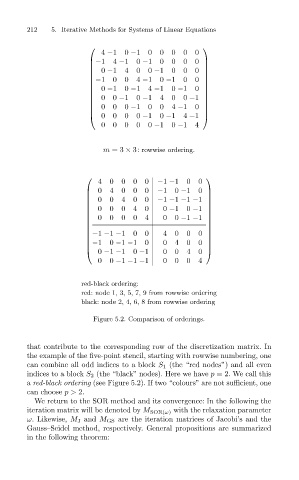
m =3 × 3: rowwise ordering.

 
4 0 0 0 0 −1 −1 0 0
 0 4 0 0 0 −1 0 −1 0 
 
 0 0 4 0 0 −1 −1 −1 −1 
 
 0 0 0 4 0 0 −1 0 −1 
 
 0 0 0 0 4 0 0 −1 −1 
 
 
−1 −1 −1 0 0 4 0 0 0
 
 
−1 0 −1 −1 0 0 4 0 0
 
 
0 −1 −1 0 −1 0 0 4 0
 
0 0 −1 −1 −1 0 0 0 4
red-black ordering:
red: node 1, 3, 5, 7, 9 from rowwise ordering
black: node 2, 4, 6, 8 from rowwise ordering
Figure 5.2. Comparison of orderings.

that contribute to the corresponding row of the discretization matrix. In
the example of the five-point stencil, starting with rowwise numbering, one
can combine all odd indices to a block S 1 (the “red nodes”) and all even
indices to a block S 2 (the “black” nodes). Here we have p = 2.We callthis
a red-black ordering (see Figure 5.2). If two “colours” are not sufficient, one
can choose p> 2.
We return to the SOR method and its convergence: In the following the
iteration matrix will be denoted by M SOR(ω) with the relaxation parameter
ω. Likewise, M J and M GS are the iteration matrices of Jacobi’s and the
Gauss–Seidel method, respectively. General propositions are summarized
in the following theorem: