Page 145 - Numerical methods for chemical engineering

The QR method for computing all eigenvalues 131

Thus, we have an orthogonal matrix P = Q [1] such that Q [1] A,
   
| | | |
[1] [1]
Q [1]  a (1) ... a [N]  =  Q a ... Q a
[1] [N] 
| | | |
 
R 11 R 12 ... R 1N
 0 | | 
 
=  .  (3.159)
 . . a (2,2) ... a (2,N) 
0 | |
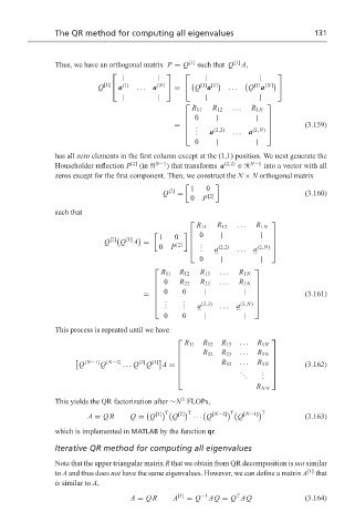
has all zero elements in the first column except at the (1,1) position. We next generate the
Householder reflection P [2] (in N−1 ) that transforms a (2,2) ∈ N−1 into a vector with all
zeros except for the first component. Then, we construct the N × N orthogonal matrix

1 0
[2]
Q = [2] (3.160)
0 P
such that
 
R 11 R 12 ... R 1N
 0 | | 
1 0
[2]
[1]

Q Q A = [2]  
 .
0 P  . . a (2,2) ... a (2,N) 

0 | |
 
R 11 R 12 R 13 ... R 1N
 0 ...
R 22 R 23 R 2N 
 
 0 0 | | 
=   (3.161)
 . . 
 . . . . a (3,3) ... a (3,N) 
0 0 | |
This process is repeated until we have
 
R 11 R 12 R 13 ... R 1N
...
R 22 R 23 R 2N
 
 
[N−1] [N−2] [2] [1]  ... 
Q Q ... Q Q A =  R 33 R 3N  (3.162)
 . . . . 
 . . 
R NN
3
This yields the QR factorization after ∼N FLOPs,

[1] T [2] T [N−2] T [N−1] T

A = QR Q = Q Q ··· Q Q (3.163)
which is implemented in MATLAB by the function qr.
Iterative QR method for computing all eigenvalues
Note that the upper triangular matrix R that we obtain from QR decomposition is not similar
to A and thus does not have the same eigenvalues. However, we can define a matrix A [1] that
is similar to A,
T
A = QR A [1] = Q −1 AQ = Q AQ (3.164)