Page 143 - Numerical methods for chemical engineering

The QR method for computing all eigenvalues 129

Inverse inflation and shift operations to find other eigenvalues

Rather than finding the eigenvalue of largest modulus, let us find the eigenvalue λ j of A
closest to some target shift value µ. As the eigenvalues of (A − µI) are λ j − µ, we only
need to derive a method that finds the smallest magnitude eigenvalue of (A − µI). We do
so by applying the iterative rule
z [k]
[k] [k] [k+1]
(A − µI)z = v v = (3.146)
z
[k]
This method can be written as
−1 [k]
(A − µI) v
v [k+1] = (3.147)
(A − µI) v
−1 [k]
−1
Thus, it returns the largest modulus eigenvalue of (A − µI) . As the eigenvalues of (A
−1
− µI) −1 are (λ j − µ) , this method finds the eigenvalue of smallest |λ j − µ|. At each
[k]
iteration, we must solve a linear system (A − µI)z [k] = v , which is done efficiently by
LU decomposition, so that later iterations only require solving two triangular systems by
substitution.
The QR method for computing all eigenvalues

We next consider a method to compute all eigenvalues of a matrix concurrently by transform-
ing the matrix into a similar one whose eigenvalues are easy to calculate. The transformation
is done through iterative use of QR decompositions, described below.

QR decomposition of a real matrix

Just as a matrix may be factored into the product of lower and upper triangular matrices, it
−1
T
may also be factored into the product of an orthogonal matrix Q, Q = Q , and an upper
triangular matrix R,
A = QR (3.148)

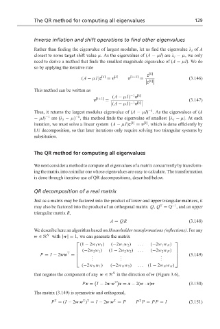
We describe here an algorithm based on Householder transformations (reflections). For any
N
w ∈ with |w|= 1, we can generate the matrix
 
(1 − 2w 1 w 1 ) (−2w 1 w 2 ) ... (−2w 1 w N )
(−2w 2 w 1 ) (1 − 2w 2 w 2 ) ... (−2w 2 w N )
 
T  
. . . (3.149)
. . .
P = I − 2ww =  
 . . . 
(−2w N w 1 ) (−2w N w 2 ) ... (1 − 2w N w N )
N
that negates the component of any w ∈ in the direction of w (Figure 3.6),
T
Px = I − 2ww x = x − 2(w · x)w (3.150)
The matrix (3.149) is symmetric and orthogonal,
T
T
T T
T
P = (I − 2ww ) = I − 2ww = P P P = PP = I (3.151)