Page 138 - Numerical methods for chemical engineering

124 3 Matrix eigenvalue analysis

e=
- 1.8284
3.8284
3.0000
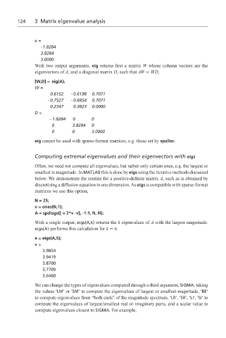
With two output arguments, eig returns first a matrix W whose column vectors are the
eigenvectors of A, and a diagonal matrix D, such that AW = WD,

[W,D] = eig(A),
W=
0.6152 - 0.6198 0.7071
- 0.7527 - 0.6854 0.7071
0.2347 0.3823 0.0000
D=
- 1.8284 0 0
0 3.8284 0
0 0 3.0000
eig cannot be used with sparse-format matrices, e.g. those set by spalloc.

Computing extremal eigenvalues and their eigenvectors with eigs
Often, we need not compute all eigenvalues, but rather only certain ones, e.g. the largest or
smallest in magnitude. In MATLAB this is done by eigs using the iterative methods discussed
below. We demonstrate the routine for a positive-definite matrix A, such as is obtained by
discretizing a diffusion equation in one dimension. As eigs is compatible with sparse-format
matrices we use this option,
N = 25;
v = ones(N,1);
A = spdiags([-v 2*v -v], -1:1, N, N);
With a single output, eigs(A,k) returns the k eigenvalues of A with the largest magnitude.
eigs(A) performs this calculation for k = 6.
e = eigs(A,5);
e=
3.9854
3.9419
3.8700
3.7709
3.6460
We can change the types of eigenvalues computed through a third argument, SIGMA, taking
the values ‘LM’ or ‘SM’ to compute the eigenvalues of largest or smallest magnitude, ‘BE’
to compute eigenvalues from “both ends” of the magnitude spectrum, ‘LR’, ‘SR’, ‘LI’, ‘SI’ to
compute the eigenvalues of largest/smallest real or imaginary parts, and a scalar value to
compute eigenvalues closest to SIGMA. For example,