Page 253 - Offshore Electrical Engineering Manual
P. 253
240    CHAPTER 6  Calculation of Load Flow, Fault Currents


                            In the calculation of the maximum short circuit currents, a voltage factor c is
                         assumed (from IEC60038) for c max,  for Low (Table 1), Medium (Table 2) and High
                         (Table 3) voltage levels. According to Fig. 4.6.1, in the case of balanced short cir-
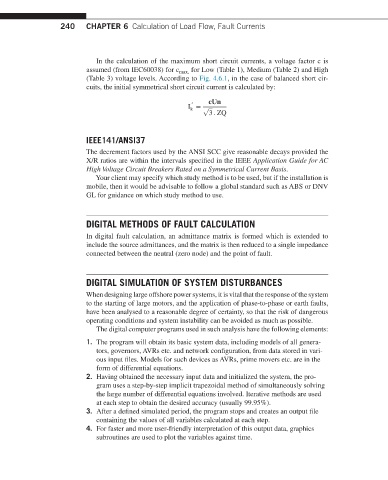
                         cuits, the initial symmetrical short circuit current is calculated by:

                                                           cUn
                                                      ″
                                                     I = √
                                                      k
                                                           3 . ZQ
                         IEEE141/ANSI37

                         The decrement factors used by the ANSI SCC give reasonable decays provided the
                         X/R ratios are within the intervals specified in the IEEE Application Guide for AC
                         High Voltage Circuit Breakers Rated on a Symmetrical Current Basis.
                            Your client may specify which study method is to be used, but if the installation is
                         mobile, then it would be advisable to follow a global standard such as ABS or DNV
                         GL for guidance on which study method to use.


                         DIGITAL METHODS OF FAULT CALCULATION
                         In digital fault calculation, an admittance matrix is formed which is extended to
                         include the source admittances, and the matrix is then reduced to a single impedance
                         connected between the neutral (zero node) and the point of fault.


                         DIGITAL SIMULATION OF SYSTEM DISTURBANCES
                         When designing large offshore power systems, it is vital that the response of the system
                         to the starting of large motors, and the application of phase-to-phase or earth faults,
                         have been analysed to a reasonable degree of certainty, so that the risk of dangerous
                         operating conditions and system instability can be avoided as much as possible.
                            The digital computer programs used in such analysis have the following elements:

                           1.   The program will obtain its basic system data, including models of all genera-
                            tors, governors, AVRs etc. and network configuration, from data stored in vari-
                            ous input files. Models for such devices as AVRs, prime movers etc. are in the
                            form of differential equations.
                           2.   Having obtained the necessary input data and initialized the system, the pro-
                            gram uses a step-by-step implicit trapezoidal method of simultaneously solving
                            the large number of differential equations involved. Iterative methods are used
                            at each step to obtain the desired accuracy (usually 99.95%).
                           3.   After a defined simulated period, the program stops and creates an output file
                            containing the values of all variables calculated at each step.
                           4.   For faster and more user-friendly interpretation of this output data, graphics
                            subroutines are used to plot the variables against time.

