Page 210 - Optofluidics Fundamentals, Devices, and Applications

Adaptive Optofluidic Devices 185

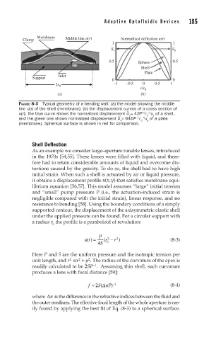
Membrane Middle line u(r)
Clamp Normalized deflection u(r)
1 1
~ ~
u s u p
0.5 Sphere 0.5
Shell
Plate
Inlet
Support
0 0
2r 0 –1 –0.5 0 0.5 1
r/r 0
(a) (b)
FIGURE 8-3 Typical geometry of a bending wall: (a) the model showing the middle
line u(r) of the shell (membrane); (b) the displacement curves of a cross section of
~
−1 - −2
u(r); the blue curve shows the normalized displacement u = 4SP r u of a shell,
~ s 0 s
−1 - −4
and the green one shows normalized displacement u = 64DP r u of a plate
s 0 p
(membrane). Spherical surface is shown in red for comparison.
Shell Deflection
As an example we consider large-aperture tunable lenses, introduced
in the 1970s [54,55]. These lenses were filled with liquid, and there-
fore had to retain considerable amounts of liquid and overcome dis-
tortions caused by the gravity. To do so, the shell had to have high
initial strain. When such a shell is actuated by air or liquid pressure,
it obtains a displacement profile ux y(, ) that satisfies membrane equi-
librium equation [56,57]. This model assumes “large” initial tension
and “small” pump pressure P (i.e., the actuation-induced strain is
negligible compared with the initial strain), linear response, and no
resistance to bending [58]. Using the boundary conditions of a simply
supported contour, the displacement of the axisymmetric elastic shell
under the applied pressure can be found. For a circular support with
a radius r the profile is a paraboloid of revolution:
0

ur() = P r ( 2 − r ) (8-3)
2
4 S 0
Here P and S are the uniform pressure and the isotropic tension per
unit length, and r ≡ x + y . The radius of the curvature of the apex is
2
2
2
−
1
readily calculated to be 2SP . Assuming thin shell, such curvature
produces a lens with focal distance [59]:
f ≈ 2 (Δ −1 (8-4)
S nP)
where Δn is the difference in the refractive indices between the fluid and
the outer medium. The effective focal length of the whole aperture is eas-
ily found by applying the best fit of Eq. (8-3) to a spherical surface.