Page 49 - Petrology of Sedimentary Rocks

poorest sorted sediments, such as glacial tills, mudflows, etc., have a, values in the
neighborhood of .!$I to 8 or even IO+.

Measures of Skewness or Asymmetry

Curves may be similar in average size and in sorting but one may be symmetrical,
the other asymmetrical. Skewness measures the degree of asymmetry as well as the
‘tsignlf-- i.e., whether a curve has an asymmetrical tail on the left or right.

Phi Quartile Skewness (Skq@). This is found by (425 + $75 - 2(Md$))/2. A (+> value
indicates that the sediment has an excess amount of fines (the frequency curve shows a
tail on the right) and a (-) value indicates a tail in the coarse (left>. The disadvantage
of this measure is that it measures only the skewness in the central part of the curve,
thus is very insensitive; also, it is greatly affected by sorting so is not a “pure” measure
of skewness. In two curves with the same amount of asymmetry, one with poor sorting
will have a much higher quartile skewness than a well-sorted sample.

Graphic Skewness. As a measure of skewness, the Graphic Skewness (SkG) given

by the formula
9 I6$.&84$~50

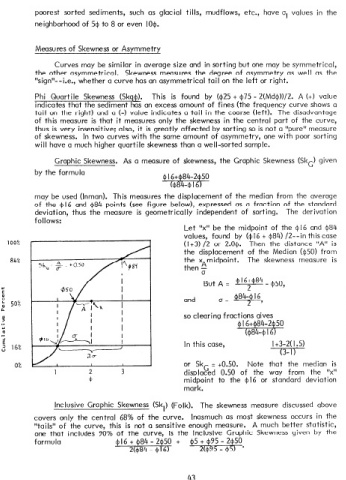
may be used (Inman). This measures the displacement of the median from the average
of the $16 and $84 points (see figure below), expressed as a fraction of the standard
deviation, thus the measure is geometrically independent of sorting. The derivation

Let “x” be the midpoint of the $16 and $84
values, found by ($ I6 + $84) /2--in this case
100% (I +3) /2 or 2.0$. Then the distance “A” is
the displacement of the Median ($50) from
84% the xAmidpoint. The skewness measure is
then a

But A = 4 ’ y4 - 050,

and o= 4@+-gW,

so clearing fractions gives

In this case, I +3-2( I .5)
-7m--
0% Or skG = +0.50. Note that the median is
displaced 0.50 of the way from the “x”
midpoint to the $ I6 or standard deviation
mark.

lnctusive Graphic Skewness (Sk,) (Folk). The skewness measure discussed above
covers only the central 68% of the curve. Inasmuch as most skewness occurs in the
“tails” of the curve, this is not a sensitive enough measure. A much better statistic,
one that includes 90% of the curve, is the Inclusive Graphic Skewness given by the
formula

43