Page 52 - Petrology of Sedimentary Rocks

than the graphic methods, which rely on only a few selected percentage lines. For
example, the median is obtained graphically by merely reading the diameter at the 50%
mark of the cumulative curve, and is not at all affected by the character of the rest of
---
the curve; but the mean, computed by the method of moments, is affected by the
distribution over every part of the curve (see sheet at the end giving graphic
significance of measures). Details on the computations involved are given in Krumbein
and Pettijohn, and many computer programs are available for calculation of these values
very rapidly. It is possible to obtain skewness and kurtosis also by means of moments,
but we will confine ourselves to determination of the mean and standard deviation. To
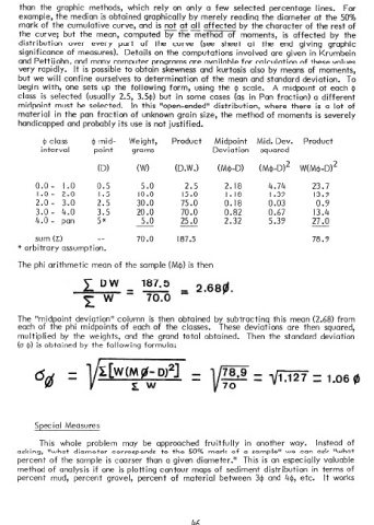
begin with, one sets up the following form, using the $I scale. A midpoint of each 0
class is selected (usually 2.5, 3.541) but in some cases (as in Pan fraction) a different
midpoint must be selected. In this “open-ended” distribution, where there is a lot of
material in the pan fraction of unknown grain size, the method of moments is severely
handicapped and probably its use is not justified.

c$ class Q rnid- Weight, Product Midpoint Mid. Dev. Product
interval point grams Deviation squared

CD> (W) (D.W .I (M@-D) (M$-D12 W(M$-D12

o.o- 1.0 0.5 5.0 2.5 2.18 4.74 23.7
I.18
0.9
3’0
:*:: 20 :*; 30.0 10.0 75.0 15.0 0.18 0.03 1.39 13.9
3:o - 4:o 3:5 20.0 70.0 0.82 0.67 13.4
4.0 - pan 5* 5.0 25.0 2.32 5.39 27.0
sum (C) -- 70.0 187.5 78.9
* arbitrary assumption.

The phi arithmetic mean of the sample (MC)) is then
z DW 187.5 2,689.

= 70.0 =

The “midpoint deviation” column is then obtained by subtracting this mean (2.68) from
each of the phi midpoints of each of the classes. These deviations are then squared,
multiplied by the weights, and the grand total obtained. Then the standard deviation
(a (11 is obtained by the following formula:

6 ;r[W(M$- D)2] - = v* = 1.06 8

pl=V zw -

Special Measures

This whole problem may be approached fruitfully in another way. Instead of
asking, “what diameter corresponds to the 50% mark of a sample” we can ask “what
percent of the sample is coarser than a given diameter.” This is an especially valuable
method of analysis if one is plotting contour maps of sediment distribution in terms of
percent mud, percent gravel, percent of material between 3$ and 44, etc. It works

46