Page 133 - Phase Space Optics Fundamentals and Applications

114 Chapter Four

*
(1) r (x, x') = f (x + x'/2) f (x + x'/2) (2)
f
F {x' → ξ} F {x → ξ'}

F –1 {ξ → x'} F –1 {ξ' → x}
W A
W (x, ξ) f(x) A (ξ', x')
f
f
→ (√ξ' + x' ,θ) }
W –1 A –1 2 2 p
–1 {(√ξ' + x' , θ) → x }
R θ = pπ/2 |F p | 2 {x→x θ } θ
F {x θ 2 p
R –1 2
θ
f
(3) RW (x , θ) F (4)
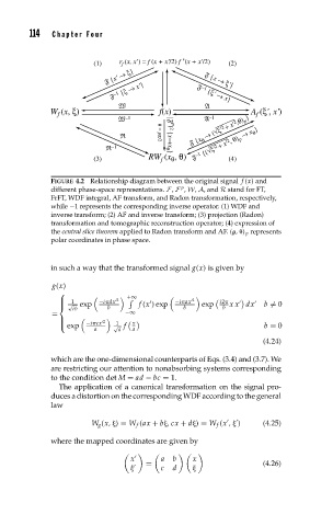
FIGURE 4.2 Relationship diagram between the original signal f (x) and
p
different phase-space representations. F, F , W, A, and R stand for FT,
FrFT, WDF integral, AF transform, and Radon transformation, respectively,
while −1 represents the corresponding inverse operator. (1) WDF and
inverse transform; (2) AF and inverse transform; (3) projection (Radon)
transformation and tomographic reconstruction operator; (4) expression of
the central slice theorem applied to Radon transform and AF. ( , ) p represents
polar coordinates in phase space.

in such a way that the transformed signal g(x) is given by

g(x)
⎧
+∞
⎪ 1 −i dx 2 −i ax 2 i2

⎪ √ exp f (x ) exp exp xx dx b = 0

⎨ b b b
ib
= −∞

⎪ 2
⎪ −i cx 1 x
⎩ exp √ f b = 0
a a a
(4.24)
which are the one-dimensional counterparts of Eqs. (3.4) and (3.7). We
are restricting our attention to nonabsorbing systems corresponding
to the condition det M = ad − bc = 1.
The application of a canonical transformation on the signal pro-
duces a distortion on the corresponding WDF according to the general
law

W g (x, ) = W f (ax + b ,cx + d ) = W f (x , ) (4.25)
where the mapped coordinates are given by

x a b x
= (4.26)
c d