Page 138 - Phase Space Optics Fundamentals and Applications

The Radon-Wigner Transform 119

Cylindrical
lens
1D input FrFT of order p
y
0 y Focal
line
x
0
x

S
Rp
z

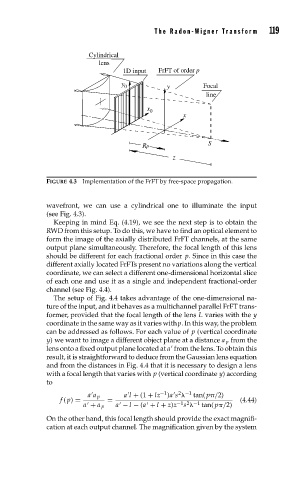
FIGURE 4.3 Implementation of the FrFT by free-space propagation.

wavefront, we can use a cylindrical one to illuminate the input
(see Fig. 4.3).
Keeping in mind Eq. (4.19), we see the next step is to obtain the
RWD from this setup. To do this, we have to find an optical element to
form the image of the axially distributed FrFT channels, at the same
output plane simultaneously. Therefore, the focal length of this lens
should be different for each fractional order p. Since in this case the
different axially located FrFTs present no variations along the vertical
coordinate, we can select a different one-dimensional horizontal slice
of each one and use it as a single and independent fractional-order
channel (see Fig. 4.4).
The setup of Fig. 4.4 takes advantage of the one-dimensional na-
ture of the input, and it behaves as a multichannel parallel FrFT trans-
former, provided that the focal length of the lens L varies with the y
coordinate in the same way as it varies withp. In this way, the problem
can be addressed as follows. For each value of p (vertical coordinate
y) we want to image a different object plane at a distance a p from the
lens onto a fixed output plane located at a from the lens. To obtain this

result, it is straightforward to deduce from the Gaussian lens equation
and from the distances in Fig. 4.4 that it is necessary to design a lens
with a focal length that varies with p (vertical coordinate y) according
to
−1
2 −1
a l + (1 + lz )a s

a a p tan( p /2)
f ( p) = = (4.44)
−1 2 −1
a + a p a − l − (a + l + z)z s tan( p /2)
On the other hand, this focal length should provide the exact magnifi-
cation at each output channel. The magnification given by the system