Page 139 - Phase Space Optics Fundamentals and Applications

120 Chapter Four

Cylindrical
lens
1D input FrFT of order p
y 0 y
Varifocal
y lens (L) Output
plane
x 0 y(R ) y
0
x
y(R )
0
x y(R )
0
x
R p
z
a p
l
a'
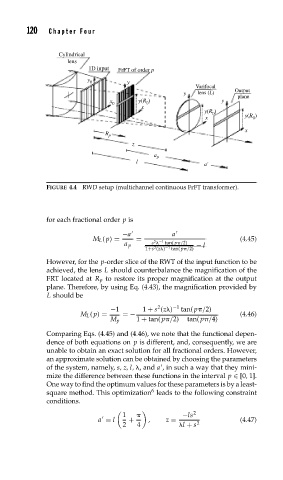
FIGURE 4.4 RWD setup (multichannel continuous FrFT transformer).

for each fractional order p is
−a a
M L ( p) = = s tan( p /2) (4.45)
2 −1
a p − l
1+s (z ) −1 tan( p /2)
2
However, for the p-order slice of the RWT of the input function to be
achieved, the lens L should counterbalance the magnification of the
FRT located at R p to restore its proper magnification at the output
plane. Therefore, by using Eq. (4.43), the magnification provided by
L should be
2
−1 1 + s (z ) −1 tan( p /2)
M L ( p) = =− (4.46)
M p 1 + tan( p /2) tan( p /4)
Comparing Eqs. (4.45) and (4.46), we note that the functional depen-
dence of both equations on p is different, and, consequently, we are
unable to obtain an exact solution for all fractional orders. However,
an approximate solution can be obtained by choosing the parameters

of the system, namely, s, z, l, , and a , in such a way that they mini-
mize the difference between these functions in the interval p ∈ [0, 1].
One way to find the optimum values for these parameters is by a least-
6
square method. This optimization leads to the following constraint
conditions.
2
1 −ls
a = l + , z = (4.47)

2 4 l + s 2