Page 187 - Phase Space Optics Fundamentals and Applications

168 Chapter Five

n
Wigner distribution function
x
y
Product space representation
y
x
Ambiguity function
m
y

x
(a)
Product space representation

(b)

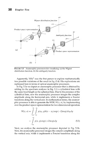
FIGURE 5.3 Anamorphic processors for visualizing: (a) the Wigner
distribution function, (b) the ambiguity function.

9
Apparently, Ville was the first person to explore mathematically
two possible variations of the result in Eq. (5.4). His explorations are
rephrased here in terms of optical anamorphic processors.
In Fig. 5.3a we depict an anamorphic processor that is obtained by
adding (to the spectrum analyzer in Fig. 5.1) a cylindrical lens with
the same focal length as the spherical lens. Due to the presence of the
cylindrical lens, now the anamorphic processor images the complex
amplitude along the horizontal axis, while it implements a Fourier
transform along the vertical axis. In mathematical terms, the anamor-
phic processor is able to generate the WDF, W(x, ), by implementing
over the product-space representation the two-dimensional operation
∞
∞
W(x, ) = p(x 0 ,y) (x − x 0 ) exp (−i2 y) dx 0 dy
−∞ −∞
∞

= p(x, y) exp (−i2 y) dy (5.5)
−∞
Next, we analyze the anamorphic processor depicted in Fig. 5.3b.
Now, the anamorphic processor images the complex amplitude along
the vertical axis, while it implements a Fourier transform along the