Page 186 - Phase Space Optics Fundamentals and Applications

Imaging Systems: Phase-Space Representations 167

n
y

X

y = 2x + X y = –2x + X

x m
–X/2 X/2

y = –2x – X y = 2x – X

– X

(a) (b)

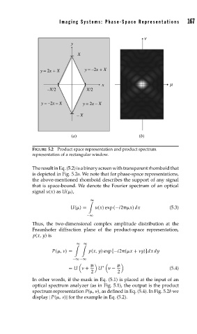
FIGURE 5.2 Product space representation and product spectrum
representation of a rectangular window.

The result in Eq. (5.2) is a binary screenwithtransparent rhomboidthat
is depicted in Fig. 5.2a. We note that for phase-space representations,
the above-mentioned rhomboid describes the support of any signal
that is space-bound. We denote the Fourier spectrum of an optical
signal u(x)as U( ),
∞

U( ) = u(x) exp (−i2 x) dx (5.3)
−∞
Thus, the two-dimensional complex amplitude distribution at the
Fraunhofer diffraction plane of the product-space representation,
p(x, y)is
∞
∞
P( , ) = p(x, y) exp [−i2 ( x + y)] dx dy
−∞ −∞

= U + U ∗ − (5.4)
2 2
In other words, if the mask in Eq. (5.1) is placed at the input of an
optical spectrum analyzer (as in Fig. 5.1), the output is the product
spectrum representation P( , ), as defined in Eq. (5.4). In Fig. 5.2b we
display |P( , )| for the example in Eq. (5.2).