Page 263 - Phase Space Optics Fundamentals and Applications

244 Chapter Eight

At any fixed z, each ray is fully characterized by its transverse po-
sition X and transverse momentum P; knowing where a ray is and in
what direction it is propagating is enough to trace it away from this
plane. This ray can then be represented by a point in the plane of x
versus p. This plane is called phase space. The complete ray family is
therefore represented by a curve, traced by the points for each ray by
varying . This curve is called the phase-space curve (PSC) or Lagrange
manifold. Notice that the integral of Eq. (8.21) gives

1 ∂ X
L(z, 1 ) − L(z, 0 ) = P(z, ) (z, ) d (8.22)
∂
0
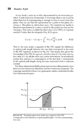
That is, the area under a segment of the PSC equals the difference
in optical path length between the rays that correspond to the ends
of the PSC segment, as shown in Fig. 8.2. This means that, given the
knowledge of the PSC for a given z and the value of L for only one ray,
the value of L for all the other rays can be determined. As mentioned
earlier, this relation is a consequence of the fact that L corresponds
to the optical path length along the rays, measured from a common
normal.
For three-dimensional fields, phase space is four-dimensional, since
there are two transverse directions and two transverse momenta. The
Lagrange manifold is then a two-parameter surface embedded in this
four-dimensional space.

p

P(z, ξ )
1
P(z, ξ )
0 L(z, ξ 0 )

–
L(z, ξ 1 )

X(z, ξ ) X(z, ξ ) x
0 1

FIGURE 8.2 The phase-space area under any segment of the PSC
corresponds to the difference in optical path length L for the corresponding
two rays.