Page 367 - Phase Space Optics Fundamentals and Applications

348 Chapter Eleven

generated by Eq. (11.20). For example, the time-frequency representa-
tion P(t, ) = I (t) ˜ I( ) is positive, and its marginals are the temporal
and spectral intensity of the pulse. 30 However, it is not uniquely re-
lated to a field and does not represent chirp properly since it is not
phase-dependent.
Coming back to bilinear time-frequency distributions, an entire
class of chronocyclic representations may be derived from the Wigner
function by means of a convolution

1

P s (t, ) = d dt W(t , )G s (t − t , − ) (11.23)
2
where
2
4 1 2 2
G s (t, ) = exp − 2 + 4 t (11.24)
s s
This class is analogous to the commonly used phase-space repre-
sentations of the optical field in quantum optics. 32,33 For s= 0, the
convolving function is a Dirac function, and P 0 is the Wigner func-
tion of the pulse. Positive values of s correspond to smoothing in
the chronocyclic space, analogous to the Q function used in quantum
physics. The time-frequency distribution defined by Eq. (11.23) is pos-
itive for s larger than 2. In the particular case of s = 2,G s is the Wigner
function of a coherent state, and P 2 corresponds to the spectrogram
of the pulse defined for coherent ensembles by Eq. (11.21), the gating
function being the Gaussian function
√
2 2
g(t) = 2 exp(− t ) (11.25)
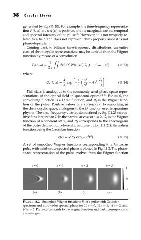
A set of smoothed Wigner functions corresponding to a Gaussian
pulse with third-order spectral phase is plotted in Fig. 11.2. The phase-
space representation of the pulse evolves from the Wigner function

s = 0 s = 1 s = 2 s = 5
1

0

–1
(a) (b) (c) (d)

FIGURE 11.2 Smoothed Wigner functions P s of a pulse with Gaussian
spectrum and third-order spectral phase for (a) s = 0, (b) s = 1, (c) s = 2, and
(d) s = 5. Part a corresponds to the Wigner function and part c corresponds to
a spectrogram.