Page 152 - Phase-Locked Loops Design, Simulation, and Applications

PLL PERFORMANCE IN THE PRESENCE OF NOISE Ronald E. Best 95

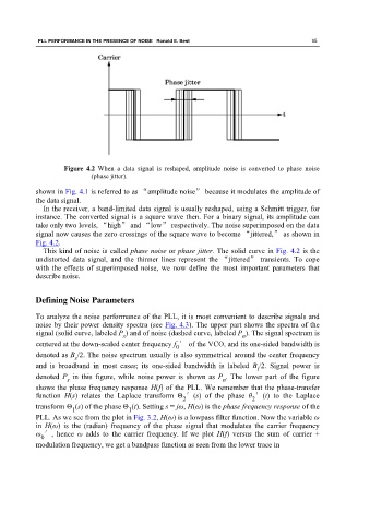
Figure 4.2 When a data signal is reshaped, amplitude noise is converted to phase noise
(phase jitter).

shown in Fig. 4.1 is referred to as “amplitude noise” because it modulates the amplitude of
the data signal.
In the receiver, a band-limited data signal is usually reshaped, using a Schmitt trigger, for
instance. The converted signal is a square wave then. For a binary signal, its amplitude can
take only two levels, “high” and “low” respectively. The noise superimposed on the data
signal now causes the zero crossings of the square wave to become “jittered,” as shown in
Fig. 4.2.
This kind of noise is called phase noise or phase jitter. The solid curve in Fig. 4.2 is the
undistorted data signal, and the thinner lines represent the “jittered” transients. To cope
with the effects of superimposed noise, we now define the most important parameters that
describe noise.

Defining Noise Parameters

To analyze the noise performance of the PLL, it is most convenient to describe signals and
noise by their power density spectra (see Fig. 4.3). The upper part shows the spectra of the
signal (solid curve, labeled P ) and of noise (dashed curve, labeled P ). The signal spectrum is
n
s
centered at the down-scaled center frequency f ′ of the VCO, and its one-sided bandwidth is
0
denoted as B /2. The noise spectrum usually is also symmetrical around the center frequency
s
and is broadband in most cases; its one-sided bandwidth is labeled B /2. Signal power is
i
denoted P in this figure, while noise power is shown as P . The lower part of the figure
s
n
shows the phase frequency response H(f) of the PLL. We remember that the phase-transfer
function H(s) relates the Laplace transform Θ ′(s) of the phase θ ′(t) to the Laplace
2 2
transform Θ (s) of the phase Θ (t). Setting s = jω, H(ω) is the phase frequency response of the
1
1
PLL. As we see from the plot in Fig. 3.2, H(ω) is a lowpass filter function. Now the variable ω
in H(ω) is the (radian) frequency of the phase signal that modulates the carrier frequency
ω ′, hence ω adds to the carrier frequency. If we plot H(f) versus the sum of carrier +
0
modulation frequency, we get a bandpass function as seen from the lower trace in