Page 164 - Phase-Locked Loops Design, Simulation, and Applications

PLL PERFORMANCE IN THE PRESENCE OF NOISE Ronald E. Best 101
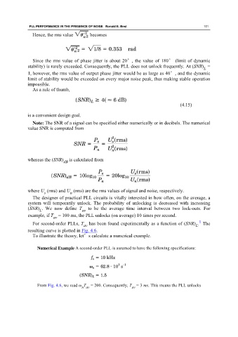
Hence, the rms value becomes

Since the rms value of phase jitter is about 20°, the value of 180° (limit of dynamic
stability) is rarely exceeded. Consequently, the PLL does not unlock frequently. At (SNR) =
L
1, however, the rms value of output phase jitter would be as large as 40°, and the dynamic
limit of stability would be exceeded on every major noise peak, thus making stable operation
impossible.
As a rule of thumb,

(4.15)

is a convenient design goal.

Note: The SNR of a signal can be specified either numerically or in decibels. The numerical
value SNR is computed from

whereas the (SNR) is calculated from
dB

where U (rms) and U (rms) are the rms values of signal and noise, respectively.
s n
The designer of practical PLL circuits is vitally interested in how often, on the average, a
system will temporarily unlock. The probability of unlocking is decreased with increasing
(SNR) . We now define T to be the average time interval between two lock-outs. For
L av
example, if T = 100 ms, the PLL unlocks (on average) 10 times per second.
av
1
For second-order PLLs, T has been found experimentally as a function of (SNR) . The
av
L
resulting curve is plotted in Fig. 4.6.
To illustrate the theory, let’s calculate a numerical example.

Numerical Example A second-order PLL is assumed to have the following specifications:

From Fig. 4.6, we read ω T = 200. Consequently, T = 3 ms. This means the PLL unlocks
n av
av