Page 83 - Phase-Locked Loops Design, Simulation, and Applications

MIXED-SIGNAL PLL ANALYSIS Ronald E. Best 58

This simple correspondence paves the way toward understanding the quite complex dynamic
performance of a PLL in the locked and unlocked states. To see what happens to a PLL when
phase and/or frequency steps of arbitrary size are applied to its reference input, we must place
the corresponding weight G(t) given by Eq. (3.50) on the platform and observe the response of
the pendulum. The notation G(t) should emphasize that G must not necessarily be a constant,
but can also be a function of time, as would be the case when an impulse is applied.
Let’s first consider the trivial case of no weight on the platform. The pendulum is then at
rest in a vertical position, φ = 0. This corresponds to the PLL operating at its center frequency
e
ω ′ with zero frequency offset (Δω = 0) and zero phase error (θ = 0).
0 e
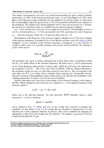
What happens if the frequency of the reference signal is changed slowly? The rate of change
of the reference frequency is assumed to be so low that the derivative term in Eq. (3.50) is
negligible. A slow variation of the reference frequency corresponds to a slow increase of
weight G, achieved by very carefully pouring a fine powder onto the platform. The analogy is
given in this case by

The pendulum now starts to deflect, indicating that a finite phase error is established within
the PLL. For small offsets of the reference frequency, the phase error θ will be proportional
e
to Δω. If the frequency offset reaches a critical value, called the hold range, the deflection of
the pendulum is just 90°. This is the static limit of stability. With the slightest disturbance,
the pendulum would now tip over and rotate around its axis forever. This corresponds to the
case where the PLL is no longer able to maintain phase tracking and consequently unlocks.
One full revolution of the pendulum equals a phase error of 2π. Because the pendulum is now
rotating permanently, the phase error increases toward infinity.
Another interesting case is given by a step change of the reference frequency at the input of
the PLL. When a frequency step of the size Δω is applied at t = 0, the angular frequency of the
reference signal is

where u(t) is the unit-step function. The first derivative therefore shows a delta
function at t = 0; this is written as

and is plotted in Fig. 3.8. What will now be the weight G(t) required to simulate this
condition? As also shown in Fig. 3.8, the weight function should be a superposition of a step
function and a delta (impulse) function. In practice, this can be simulated by dropping an
appropriate weight from some height onto the platform. The impulse is generated when the
weight hits the platform. To get

Printed from Digital Engineering Library @ McGraw-Hill (www.Digitalengineeringlibrary.com).
Copyright ©2004 The McGraw-Hill Companies. All rights reserved.
Any use is subject to the Terms of Use as given at the website.