Page 120 - Physical Principles of Sedimentary Basin Analysis

102 Burial histories

A B C D E X F G X H
0 2500
(b)
500 H
2000
1000 1500 E G H
depth [m] 1500 F ζ−coordinate [m] D

2000 1000 C F
A B
500
2500 (a)
A
3000 0
−250 −200 −150 −100 −50 0 −250 −200 −150 −100 −50 0
time [Ma] time [Ma]
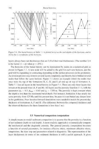
Figure 5.4. The burial history in Table 5.1 is plotted in (a) as the real depths of the horizons, and in
(b) by the ζ-coordinates of the horizons.

layers always have net thicknesses that are 3/4 of their real thicknesses. (The number 3/4
is the factor (1 − φ) when φ = 25%.)
The horizons of the burial history can be represented by nodes in a numerical grid as
showninFigure 5.3. A new node will be added to the grid for each new horizon, and the
grid will be expanding or contracting depending on the surface processes in the geohistory.
An erosion process may remove several layers completely and thereby leave behind several
nodes that follow the same horizon. Figure 5.4 shows an example where the nodes that
once were the top of the formations B, C, D, and E all end up on top of formation A.
Table 5.1 lists all layers in the burial history in Figure 5.4. There are only three layers that
remain at the present time (A, F and H). All layers use the porosity function (5.1), with the
parameters φ 0 = 0.5, φ min = 0.03 and ζ 0 = 1350 m. The porosity is kept constant when
the depth is less than the maximum burial depth. For instance, formation A has nearly the
same porosity from 125 Ma until the present time, because it is not buried any deeper later
in the geohistory. Four iterative forward simulations were needed to match the present-day
thickness of formations A, F and H. (The difference between the computed thickness and
the observed thickness for these formations is less than 1 m.)

5.5 Numerical compaction computation
A simple means to model sediment compaction is to assume that the porosity is a function
of net sediment depth (or real depth). A more realistic approach is to numerically compute
the mechanical and the diagenetic porosity. The general porosity computation becomes
a function of several parameters, for instance effective stress, maximum effective stress,
temperature, the time step and parameters related to diagenesis. The representation of the
layer thicknesses in terms of net sediment thickness is still a useful approach. It gives