Page 121 - Physical Principles of Sedimentary Basin Analysis

5.5 Numerical compaction computation 103

a Lagrangian grid, except for the surface layer, where sediments are deposited. We can
compute the real layer thicknesses for any general porosity computation from the knowl-
edge of the net amount of rock in each formation, by doing the following tasks at each time
step:

1. compute the porosity using the z-coordinates, pressure (p), temperature (T ), etc., from the
n
n
n
n
n
previous time step: φ n+1 = f (φ , z , T , p , t n+1 − t ,...);
2. compute current real layer thicknesses from the net-thicknesses and the current porosities:
z n+1 = ζ/(1 − φ n+1 );
3. make current z-coordinates by adding the layer thicknesses: z n+1 ;
4. solve equations for temperature and pressure using the current z-coordinates.
The superscripts n and n + 1 denote the previous and the current time step, respectively.
It is straightforward to iterate over the task list above, but experience shows that iterations
are unnecessary with moderate time steps. The reason is that the porosity does not change
very much from one time step to the next. The scheme above allows real thicknesses and
the z-coordinate to be computed once we know the net amount of rock in each formation.
The observed layer thicknesses are reproduced using repeated forward simulations of the
burial history as shown in the preceding section. The net amount of rock in each layer
is then updated at the end of each forward simulation using the computed present-day
porosities and the present-day layer thicknesses. Notice that there are no restrictions on
how we compute the porosities. It is difficult to prove rigorously that such a scheme con-
verges, but experience tells us that less than ten forward simulations are needed to obtain
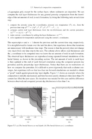
a “good” match against present-day layer depths. Figure 5.5 shows an example where the
compaction is initially mechanical, and then becomes purely chemical when more than 2%
cement has filled the pore space. Six iterations was needed for this case and the difference
between observed and computed present day thicknesses is less than 1 m.

0 J C P E O M P 3000 J C P E O M P
Nordland−fm
Naust−fm 2500
1000
Kai−fm
Hordaland−gp 2000
Tare−fm
depth [m] 2000 Tang−fm zeta−coordinate [m] 1500
Nise−fm
Kvitnos−fm
Spekk−fm
Garn−fm 1000
Not−fm
3000 Ile−fm
Ror−fm
Tilje−fm
500
Aare−fm
4000 0
−200 −150 −100 −50 0 −200 −150 −100 −50 0
time [Ma] time [Ma]
(a) (b)
Figure 5.5. (a) The burial history as real depth. (b) The burial history as ζ-coordinate.