Page 143 - Physical Principles of Sedimentary Basin Analysis

6.6 Stationary geotherms in the lithospheric mantle 125

geotherms. The first is function (6.90) and the second is the heat conductivity based on
work by Hofmeister (1999) and given by McKenzie and Jackson (2005)as

3
b n
λ H (T ) = + d n (T + 273) (6.91)
1 + cT
n=1
◦
where λ H is in units W m −1 K −1 , T is in C. The parameters are b = 5.3, c = 0.0015,
d 0 = 1.753 · 10 −2 , d 1 =−1.0365 · 10 −4 , d 2 = 2.2451 · 10 −7 , d 3 =−3.4071 · 10 −11 .The
third heat conductivity function is
n
298

λ X (T ) = λ 0 (6.92)
T + 273
which is proposed by Xu et al. (2004), where λ 0 = 4.08 W m −1 K −1 and n = 0.406.
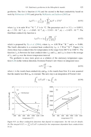
The fourth alternative is a constant heat conductivity λ B = 3W m −1 K −1 . Figure 6.9a
◦
◦
shows these heat conductivities for temperatures in the range from 200 C to 1300 C. The
function λ A is between the heat conductivities λ H and λ X , and λ B is close to the average
of λ A and λ H over the shown temperature interval.
The geotherm is once more given as a solution of the stationary temperature equa-
tion (6.20) in the vertical direction. It returns Fourier’s law when it is integrated once:
dT
λ(T ) = q m (6.93)
dz
where λ is the mantle heat conductivity and q m is the mantle heat flow. It is now assumed
that the mantle heat flow q m is constant. The next step is an integration of Fourier’s law
T z
λ(T ) dT = q m dz (6.94)
T m z m
4.5 6000
(a) (b)
5000 Xu
heat conductivity [W/mK] 3.5 B G−function [W/m] 4000 Hofmeister
4.0
Hofmeister

3000
3.0
2000
A
2.5
1000 A
Xu
B
2.0 0
200 400 600 800 1000 1200 1400 200 400 600 800 1000 1200 1400
temperature [°C] temperature [°C]
Figure 6.9. (a) Heat conductivity functions that depend on temperature. See the text for details.
T
(b) The integral G(T ) = λ(T ) dT is plotted for the temperature dependent heat conductivities
T 0
in (a).