Page 144 - Physical Principles of Sedimentary Basin Analysis

126 Heat flow

0

50

depth [km] 100 Xu

A
150
B
Hofmeister
200
0 500 1000 1500
temperature [°C]
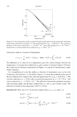
Figure 6.10. The temperature profile is plotted through the lithosphere for the temperature dependent
mantle heat conductivities in Figure 6.9. The mantle heat flow is q m = 0.02 Wm −2 . The crust has a
thickness 35 km, heat conductivity λ c = 2.5 Wm −1 K −1 and a heat production S = 10 −6 Wm −3 .
Profile B has a constant mantle heat conductivity λ m = 3 Wm −1 K −1 .

which gives depth as a function of temperature:

1 T
z = z m + (G(T ) − G(T m )) where G(T ) = λ(T ) dT. (6.95)
q m
T m
The difference in G-value for two temperatures gives the vertical distance between the
temperatures. A constant heat conductivity λ B gives a linear G-function. Figure 6.9bshows
the G-functions for the heat conductivities in Figure 6.9a, and all G-functions have a quite
similar steepness.
It is straightforward to plot the depth as a function of temperature once we have the
G-function. (See Exercise 6.12 for details.) Figure 6.10 shows the geotherms in the case of
the four different heat conductivities when the mantle heat flow is q m = 0.02 W m −2 .The
crust has a thickness z m = 35 km with a constant heat generation S 0 = 1·10 −6 Wm −3 and
a heat conductivity λ c = 2.5W m −1 K −1 . The difference between the geotherms increases
with increasing depth, and the heat conductivities λ B and λ H give similar results. The
◦
difference in depth for the temperature 1300 Cis30km.
Exercise 6.12 Show that G(T ) for the heat conductivities λ B , λ A , λ H and λ X is

G B (T ) = λ B T (6.96)
λ 0
G A (T ) = ln(1 + c 0 T ) (6.97)
c 0
3
b d n n+1
G H (T ) = ln(1 + cT ) + (T + 273) (6.98)
c (n + 1)
n=1