Page 39 - Physical Principles of Sedimentary Basin Analysis

2.8 The rotation matrix 21

z′ z

x′
α
θ
x
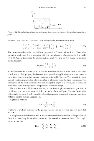
Figure 2.14. The primed coordinate frame is rotated an angle θ relative to the unprimed coordinate
frame.

because x = a cos α and z = a sin α, and using matrix notation we can write

x cos θ sin θ x x
= = R(θ) . (2.53)
z − sin θ cos θ z z
The rotation matrix can be checked by trying out θ = 0 (no rotation), θ = π/2 (rotation
◦
by a right angle) and θ = π (rotation 180 ). A special case is when the angle θ is small,
(θ
1). We can then make the approximations cos θ ≈ 1 and sin θ ≈ θ, and the rotation
matrix becomes

1 θ
R(θ) ≈ . (2.54)
−θ 1
A nice feature of the rotation matrix is that the inverse of the matrix is the same as the trans-
posed matrix. This property is time-saving in numerical applications where for instance
each finite element requires its own rotation matrix and its inverse. The numerical inver-
sion of rotation matrices for a large number of elements could be time consuming. The
application of the rotation matrix does not change the length of a vector, and it left as an
exercise to show that equation (2.53) preserves the vector length.
The rotation matrix R(θ) takes a (fixed) vector from a given coordinate system to a
coordinate system rotated an angle θ. It is seen directly from Figure 2.14 that the rotation
of the vector an angle θ with respect to a (fixed) coordinate system is the same as a rotation
of the coordinate system an angle −θ.
A gradient operator
∂ ∂
∇= n x + n z (2.55)
∂x ∂z
rotates to a gradient operator in the primed system just as a vector, and we have that

∇ = R∇.
A simple way to obtain the entries in the rotation matrix is to make the scalar products of
the unit vectors along the axes in the two respective coordinate systems. In the 2D example
above we see that

n · n x n · n z
x
x
R = (2.56)
n · n x n · n z
z
z