Page 93 - Physical Principles of Sedimentary Basin Analysis

3.22 Streamlines in 2D 75

4 4

3 3
y−coordinate [−] 2 y−coordinate [−] 2

1 1

0 0
0 0.20 0.40 0.60 0.80 1 1.20 0 1 2 3 4
x−coordinate [−] x−coordinate [−]
(a) (b)
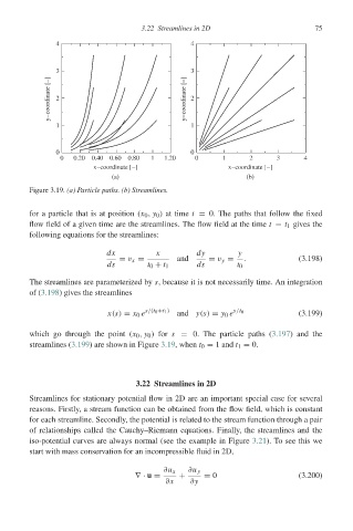
Figure 3.19. (a) Particle paths. (b) Streamlines.

for a particle that is at position (x 0 , y 0 ) at time t = 0. The paths that follow the fixed
flow field of a given time are the streamlines. The flow field at the time t = t 1 gives the
following equations for the streamlines:

dx x dy y
= v x = and = v y = . (3.198)
ds t 0 + t 1 ds t 0
The streamlines are parameterized by s, because it is not necessarily time. An integration
of (3.198) gives the streamlines

x(s) = x 0 e s/(t 0 +t 1 ) and y(s) = y 0 e s/t 0 (3.199)

which go through the point (x 0 , y 0 ) for s = 0. The particle paths (3.197) and the
streamlines (3.199) are shown in Figure 3.19, when t 0 = 1 and t 1 = 0.

3.22 Streamlines in 2D
Streamlines for stationary potential flow in 2D are an important special case for several
reasons. Firstly, a stream function can be obtained from the flow field, which is constant
for each streamline. Secondly, the potential is related to the stream function through a pair
of relationships called the Cauchy–Riemann equations. Finally, the streamlines and the
iso-potential curves are always normal (see the example in Figure 3.21). To see this we
start with mass conservation for an incompressible fluid in 2D,

∂u x ∂u y
∇· u = + = 0 (3.200)
∂x ∂y