Page 96 - Physical Principles of Sedimentary Basin Analysis

78 Linear elasticity and continuum mechanics

0.4 m/years
(a) (b)
1200 1200
−10
1000 10 15 20 25 −5 −15 −20
1.5 5 0.1 −25 1000
1.4 0.2
1.3 0.3
1.2 0.4
1.1 0.5
800 1.0 0.6 800
height [m] 600 0.9 0.8 0.7 height [m] 600
400 400
200 200
0
0 0
0 200 400 600 800 1000 0 200 400 600 800 1000
width [m] width [m]
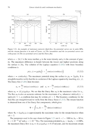
Figure 3.21. An example of stationary meteoric fluid flow. Iso-potential curves are in units MPa,
2
and the stream function is in units m /years. (a) The streamlines and the iso-potential curves are
orthogonal. (b) The iso-potential curves and the Darcy flux.

where ω = 2π/l is the wave number, is the water density and g is the constant of grav-
ity. The maximum difference in height between the lowest and highest positions along
the surface is 2h 0 . The solution of the Laplace equation (3.202) with these boundary
conditions is
1

p(x, z) = gh 0 1 + cos(ωx) cosh(ωz) (3.212)
c
where c = cosh(ωh 0 ). The maximum potential along the surface is p 0 = 2 gh 0 .Itis
straightforward to verify that this is a solution of the Laplace equation by inserting p(x, y).
The Darcy flux (3.201) then becomes

u 0 u 0
u x = sin(ωx) cosh(ωz) and u z =− cos(ωx) sinh(ωz) (3.213)
c c
where u 0 = (k/μ) gh 0 ω. We see that the Darcy flux u 0 is the maximum value for u x .
The flux u 0 is also an accurate estimate for the maximum of u z whenever sinh(ωh)/c =
tanh(ωh) ≈ 1, a condition that may be written ωh > 2. The boundary conditions for the
fluid flux are straightforward to verify from the Darcy fluxes (3.213). The stream function
is obtained from one of the Darcy flux components, which gives

0
= u x dz = sin(ωx) sinh(ωz) (3.214)
c
where 0 = k gh 0 /μ is approximately the maximum value for the stream function when
ωh > 2.
The parameters used in the case shown in Figure 3.21 are h = l = 1000 m, h 0 = 80 m,
2
k = 1·10 −15 m and μ = 1·10 −3 Pa s. The maximum potential is p 0 = 2 gh 0 = 1.6MPa,
the maximum Darcy flow is u 0 = (k/μ) gh 0 ω = 0.15 m/years, and the maximum stream