Page 324 - Physical Chemistry

lev38627_ch10.qxd 3/14/08 1:07 PM Page 305

305
10.4 ACTIVITY COEFFICIENTS ON THE MOLALITY Section 10.4
Activity Coefficients on the Molality
AND MOLAR CONCENTRATION SCALES and Molar Concentration Scales
So far in this chapter, we have expressed solution compositions using mole fractions
and have written the chemical potential of each solute i as

m m° RT ln g x where g II,i S 1 as x S 1 (10.24)
A
II,i
II,i i
i
where A is the solvent. However, for solutions of solids or gases in a liquid, the solute
chemical potentials are usually expressed in terms of molalities. The molality of solute
i is m n /n M [Eq. (9.3)]. Division of numerator and denominator by n tot gives
i
i
A
A
m x /x M and x m x M . The m expression becomes
i A
i
A
A
i
A
i
i
m m° RT ln 1g m x M m°>m°2 (10.25)
i
II,i
i A
A
II,i
m m° RT ln 1M m°2 RT ln 1x g m >m°2 (10.26)
A II,i
i
i
II,i
A
where, to keep later equations dimensionally correct, the argument of the logarithm
was multiplied and divided by m°, where m° is defined by m° 1 mol/kg. We can take
the log of a dimensionless number only. The quantity M m° is dimensionless. For
A
example, for H O, M m° (18 g/mol)
(1 mol/kg) 0.018.
A
2
We now define m° and g m,i as
m,i
m° m° RT ln 1M m°2, g m,i x g (10.27)
II,i
m,i
A
A II,i
With these definitions, m becomes
i
m m° RT ln 1g m,i m >m°2, m° 1 mol>kg, i A (10.28)*
i
m,i
i
g m,i S 1 as x S 1 (10.29)
A
where the limiting behavior of g m,i follows from (10.27) and (10.10). The motive for
the definitions in (10.27) is to produce an expression for m in terms of m that has the
i
i
same form as the expression for m in terms of x . Note the similarity between (10.28)
i
i
and (10.24). We call g m,i the molality-scale activity coefficient of solute i and m° the
m,i
molality-scale standard-state chemical potential of i. Since m° in (10.27) is a func-
II,i
tion of T and P only, m° is a function of T and P only.
m,i
What is the molality-scale standard state? Setting m in (10.28) equal to m° , we
i
m,i
see that this standard state has g m,i m /m° 1. We shall take the standard-state molal-
i
ity as m m° 1 mol/kg (as is implied in the notation m° for 1 mol/kg), and we must
i
then have g m,i 1 in the standard state. The molality-scale solute standard state is thus
the fictitious state (at the T and P of the solution) with m 1 mol/kg and g m,i 1.
i
This state involves an extrapolation of the behavior of the ideally dilute solution
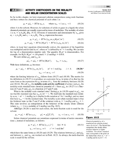
(where g m,i 1) to a molality of 1 mol/kg (see Fig. 10.5).
Although (10.28) is used for each solute, the mole-fraction scale is used for the
solvent:
m m° RT ln g x , m° m*1T, P2, g S 1 as x S 1 (10.30)
A A
A
A
A
A
A
A
Solute chemical potentials are sometimes expressed in terms of molar concentra- Figure 10.5
tions c instead of molalities, as follows: Chemical potential m of a
i
i
nonelectrolyte solution plotted
m m° RT ln 1g c >c°2 for i A (10.31) versus ln (m /m°). The dashed line
c,i i
c,i
i
i
g S 1 as x S 1 c° 1 mol>dm 3 extrapolates the ideally dilute
solution behavior to higher
c,i
A
molalities. The solute’s standard
which have the same forms as (10.28) and (10.29). The relations between m° and m°
c,i II,i state corresponds to the point on
and between g and g are worked out in Prob. 10.23. As always, the mole-fraction
c,i II,i the dashed line where m m°
i
scale is used for the solvent. 1 mol/kg and ln (m /m°) 0.
i