Page 372 - Physical Chemistry

lev38627_ch12.qxd 3/18/08 2:41 PM Page 353

353
The solution’s freezing point T is a function of the activity a of A in solution. Section 12.3
f
A
Alternatively, we can consider T to be the independent variable and view a as a func- Freezing-Point Depression and
f
A
Boiling-Point Elevation
tion of T .Wenow differentiate (12.4) with respect to T at constant P.In Chapter 6, we
f
f
differentiated ln K° G°/RT [Eq. (6.14)] with respect to T to get (d/dT)(ln K°)
P
P
2
(d/dT)( G°/RT) H°/RT [Eq. (6.36)] for a chemical reaction. We can consider
the fusion process A(s) → A(l) at pressure P° and temperature T as a reaction with
f
A(s) as the reactant and A(l) as the product. Therefore the same derivation that gave A(sln) B(sln)
2
d( G°/RT)/dT H°/RT can be applied to the fusion process to give
d ¢ G m,A 1T 2 ¢ H m,A 1T 2
fus
fus
f
f
a b A(s) T T f
dT f RT f RT f 2
Taking ( / T ) of (12.4), we thus get
f
0 ln a A ¢ H m,A 1T 2 A(l)
fus
f
a b (12.5)
0T f P RT f 2
A(s)
2

d ln a 1¢ H m,A >RT 2 dT P const. (12.6)
fus
f
A
f
T T* f
where H m,A (T ) is the molar enthalpy of fusion of pure A at T and 1 atm. [Since
f
fus
f
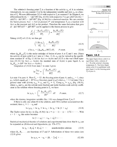
the activity of pure solid A at 1 atm is 1 (Sec. 11.4), a can be viewed as the equilib- Figure 12.3
A
rium constant K° of Eq. (11.6) for A(s) ∆ A(sln) and (12.5) is the van’t Hoff equa- The upper figure shows solid A in
tion (11.32) for A(s) ∆ A(sln); the standard state of A(sln) is pure liquid A, so equilibrium with a solution of
H m,A is H° for A(s) ∆ A(sln).] A B at the solution’s freezing
fus
Integration of (12.6) from state 1 to state 2 gives temperature T . The lower figure
f
shows solid A in equilibrium with
a A,2 2 ¢ H m,A 1T 2 pure liquid A at the freezing point
fus
f
ln dT f T* of pure A.
f
a RT 2
A,1
1 f
Let state 1 be pure A. Then T T*, the freezing point of pure A, and a A,1 1, since
f,1
f
m (which equals m* RT ln a ) becomes equal to m* when a 1. Let state 2 be a
A
A
A
A
A
general state with activity a A,2 a and T f,2 T . Using a g x [Eq. (10.5)],
A
A
A A
f
where x and g are the solvent mole fraction and mole-fraction-scale activity coeffi-
A
A
cient in the solution whose freezing point is T , we have
f
A A T f ¢ H m,A 1T2
fus
ln g x dT P const. (12.7)
RT 2
T * f
where the dummy integration variable (Sec. 1.8) was changed from T to T.
f
If there is only one solute B in the solution, and if B is neither associated nor dis-
sociated, then x 1 x and
B
A
ln g x ln g ln x ln g ln 11 x 2 (12.8)
A
A A
A
B
A
2
The Taylor series for ln x is [Eq. (8.36)]: ln x (x 1) (x 1) /2 . With
x 1 x , this series becomes
B
ln 11 x 2 x x >2 . . .
2
B
B
B
Statistical-mechanical theories of solutions and experimental data show that ln g can
A
be expanded as (Kirkwood and Oppenheim, pp. 176–177):
3
2
ln g B x B x p nonelectrolyte solution (12.9)
2 B
3 B
A
where B , B , . . . are functions of T and P. Substitution of these two series into
2
3
(12.8) gives
1
ln g x x 1B 2x . . . (12.10)
2
B
A A
2
B
2